Hello! I'm kicking off another article series about the internals of PostgreSQL. This one will focus on query planning and execution mechanics.
This series will cover:
Query execution stages (this article)
Statistics
Sequential scan
Index scan
Nested-loop join
Hash join
Merge join
This article borrows from our course QPT Query Optimization (available in English soon), but focuses mostly on the internal mechanisms of query execution, leaving the optimization aspect aside. Please also note that this article series is written with PostgreSQL 14 in mind.
Simple query protocol
The fundamental purpose of the PostgreSQL client-server protocol is twofold: it sends SQL queries to the server, and it receives the entire execution result in response. The query received by the server for execution goes through several stages.
Parsing
First, the query text is parsed, so that the server understands exactly what needs to be done.
Lexer and parser. The lexer is responsible for recognizing lexemes in the query string (such as SQL keywords, string and numeric literals, etc.), and the parser makes sure that the resulting set of lexemes is grammatically valid. The parser and lexer are implemented using the standard tools Bison and Flex.
The parsed query is represented as an abstract syntax tree.
Example:
SELECT schemaname, tablename
FROM pg_tables
WHERE tableowner = 'postgres'
ORDER BY tablename;
Here, a tree will be built in backend memory. The figure below shows the tree in a highly simplified form. The nodes of the tree are labeled with the corresponding parts of the query.

RTE is an obscure abbreviation that stands for "Range Table Entry." The name "range table" in the PostgreSQL source code refers to tables, subqueries, results of joins–in other words, any record sets that SQL statements operate on.
Semantic analyzer. The semantic analyzer determines whether there are tables and other objects in the database that the query refers to by name, and whether the user has the right to access these objects. All the information required for semantic analysis is stored in the system catalog.
The semantic analyzer receives the parse tree from the parser and rebuilds it, supplementing it with references to specific database objects, data type information, etc.
If the parameter debug_print_parse is on, the full tree will be displayed in the server message log, although there is little practical sense in this.
Transformation
Next, the query can be transformed (rewritten).
Transformations are used by the system core for several purposes. One of them is to replace the name of a view in the parse tree with a subtree corresponding to the query of this view.
pg_tables from the example above is a view, and after transformation the parse tree will take the following form:
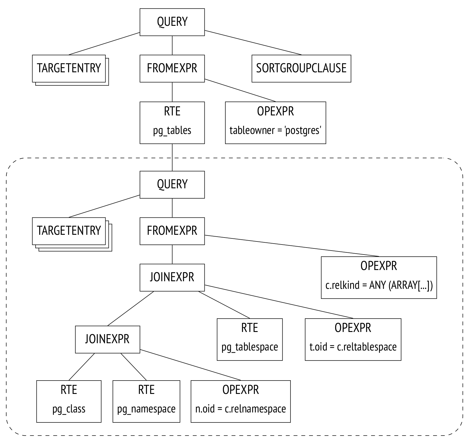
This parse tree corresponds to the following query (although all manipulations are performed only on the tree, not on the query text):
SELECT schemaname, tablename
FROM (
    -- pg_tables
    SELECT n.nspname AS schemaname,
      c.relname AS tablename,
      pg_get_userbyid(c.relowner) AS tableowner,
      ...
    FROM pg_class c
      LEFT JOIN pg_namespace n ON n.oid = c.relnamespace
      LEFT JOIN pg_tablespace t ON t.oid = c.reltablespace
    WHERE c.relkind = ANY (ARRAY['r'::char, 'p'::char])
)
WHERE tableowner = 'postgres'
ORDER BY tablename;
The parse tree reflects the syntactic structure of the query, but not the order in which the operations will be performed.
Row-level security is implemented at the transformation stage.
Another example of the use of transformations by the system core is the implementation of SEARCH and CYCLE clauses for recursive queries in version 14.
PostgreSQL supports custom transformations, which the user can implement using the rewrite rule system.
The rule system was intended as one of the primary features of Postgres. The rules were supported from the project's foundation and were repeatedly redesigned during early development. This is a powerful mechanism but difficult to understand and debug. There was even a proposal to remove the rules from PostgreSQL entirely, but it did not find general support. In most cases, it is safer and more convenient to use triggers instead of rules.
If the parameter debug_print_rewritten is on, the complete transformed parse tree will be displayed in the server message log.
Planning
SQL is a declarative language: a query specifies what to retrieve, but not how to retrieve it.
Any query can be executed in a number of ways. Each operation in the parse tree has multiple execution options. For example, you can retrieve specific records from a table by reading the whole table and discarding rows you don't need, or you can use indexes to find the rows that match your query. Data sets are always joined in pairs. Variations in the order of joins result in a multitude of execution options. Then there are various ways to join two sets of rows together. For example, you could go through the rows in the first set one by one and look for matching rows in the other set, or you could sort both sets first, and then merge them together. Different approaches perform better in some cases and worse in others.
The optimal plan may execute faster than a non-optimal one by several orders of magnitude. This is why the planner, which optimizes the parsed query, is one of the most complex elements of the system.
Plan tree. The execution plan can also be presented as a tree, but with its nodes as physical rather than logical operations on data.

If the parameter debug_print_plan is on, the full plan tree will be displayed in the server message log. This is highly impractical, as the log is extremely cluttered as it is. A more convenient option is to use the EXPLAIN command:
EXPLAIN
SELECT schemaname, tablename
FROM pg_tables
WHERE tableowner = 'postgres'
ORDER BY tablename;
                            QUERY PLAN
−−−−−−−−−−−−−−−−−−−−−−−−−−−−−−−−−−−−−−−−−−−−−−−−−−−−−−−−−−−−−−−−−−−−−
 Sort  (cost=21.03..21.04 rows=1 width=128)
   Sort Key: c.relname
   −> Nested Loop Left Join  (cost=0.00..21.02 rows=1 width=128)
       Join Filter: (n.oid = c.relnamespace)
       −> Seq Scan on pg_class c  (cost=0.00..19.93 rows=1 width=72)
           Filter: ((relkind = ANY ('{r,p}'::"char"[])) AND (pg_g...
       −> Seq Scan on pg_namespace n  (cost=0.00..1.04 rows=4 wid...
(7 rows)
The image shows the main nodes of the tree. The same nodes are marked with arrows in the EXPLAIN output.
The Seq Scan node represents the table read operation, while the Nested Loop node represents the join operation. There are two interesting points to take note of here:
One of the initial tables is gone from the plan tree because the planner figured out that it's not required to process the query and removed it.
There is an estimated number of rows to process and the cost of processing next to each node.
Plan search. To find the optimal plan, PostgreSQL utilizes the cost-based query optimizer. The optimizer goes through various available execution plans and estimates the required amounts of resources, such as I/O operations and CPU cycles. This calculated estimate, converted into arbitrary units, is known as the plan cost. The plan with the lowest resulting cost is selected for execution.
The trouble is, the number of possible plans grows exponentially as the number of joins increases, and sifting through all the plans one by one is impossible even for relatively simple queries. Therefore, dynamic programming and heuristics are used to limit the scope of search. This allows to precisely solve the problem for a greater number of tables in a query within reasonable time, but the selected plan is not guaranteed to be truly optimal because the planner utilizes simplified mathematical models and may use imprecise initial data.
Ordering joins. A query can be structured in specific ways to significantly reduce the search scope (at a risk of missing the opportunity to find the optimal plan):
Common table expressions are usually optimized separately from the main query. Since version 12, this can be forced with the MATERIALIZE clause.
Queries from non-SQL functions are optimized separately from the main query. (SQL functions can be inlined into the main query in some cases.)
The join_collapse_limit parameter together with explicit JOIN clauses, as well as the from_collapse_limit parameter together with sub-queries may define the order of some joins, depending on the query syntax.
The last one may need an explanation. The query below calls several tables within a FROM clause with no explicit joins:
SELECT ...
FROM a, b, c, d, e
WHERE ...
This is the parse tree for this query:

In this query, the planner will consider all possible join orders.
In the next example, some joins are explicitly defined by the JOIN clause:
SELECT ...
FROM a, b JOIN c ON ..., d, e
WHERE ...
The parse tree reflects this:

The planner collapses the join tree, effectively transforming it into the tree from the previous example. The algorithm recursively traverses the tree and replaces each JOINEXPR node with a flat list of its components.
This "flattening out" will only occur, however, if the resulting flat list will contain no more than join_collapse_limit elements (8 by default). In the example above, if join_collapse_limit is set to 5 or less, the JOINEXPR node will not be collapsed. For the planner this means two things:
Table B must be joined to table C (or vice versa, the join order in a pair is not restricted).
Tables A, D, E, and the join of B to C may be joined in any order.
If join_collapse_limit is set to 1, any explicit JOIN order will be preserved.
Note that the operation FULL OUTER JOIN is never collapsed regardless of join_collapse_limit.
The parameter from_collapse_limit (also 8 by default) limits the flattening of sub-queries in a similar manner. Sub-queries don't appear to have much in common with joins, but when it comes down to the parse tree level, the similarity is apparent.
Example:
SELECT ...
FROM a, b JOIN c ON ..., d, e
WHERE ...
And here's the tree:

The only difference here is that the JOINEXPR node is replaced with FROMEXPR (hence the parameter name FROM).
Genetic search. Whenever the resulting flattened tree ends up with too many same-level nodes (tables or join results), planning time may skyrocket because each node requires separate optimization. If the parameter geqo is on (it is by default), PostgreSQL will switch to genetic search whenever the number of same-level nodes reaches geqo_threshold (12 by default).
Genetic search is much faster than the dynamic programming approach, but it does not guarantee that the best possible plan will be found. This algorithm has a number of adjustable options, but that's a topic for another article.
Selecting the best plan. The definition of the best plan varies depending on the intended use. When a complete output is required (for example, to generate a report), the plan must optimize the retrieval of all rows that match the query. On the other hand, if you only want the first several matching rows (to display on the screen, for example), the optimal plan might be completely different.
PostgreSQL addresses this by calculating two cost components. They are displayed in the query plan output after the word "cost":
Sort (cost=21.03..21.04 rows=1 width=128)The first component, startup cost, is the cost to prepare for the execution of the node; the second component, total cost, represents the total node execution cost.
When selecting a plan, the planner first checks if a cursor is in use (a cursor can be set up with the DECLARE command or explicitly declared in PL/pgSQL). If not, the planner assumes that the full output is required and selects the plan with the least total cost.
Otherwise, if a cursor is used, the planner selects a plan that optimally retrieves the number of rows equal to cursor_tuple_fraction (0.1 by default) of the total number of matching rows. Or, more specifically, a plan with the lowest
startup cost + cursor_tuple_fraction × (total cost − startup cost).
Cost calculation process. To estimate a plan cost, each of its nodes has to be individually estimated. A node cost depends on the node type (reading from a table costs much less than sorting the table) and the amount of data processed (in general, the more data, the higher the cost). While the node type is known right away, to assess the amount of data we first need to estimate the node's cardinality (the amount of input rows) and selectivity (the fraction of rows left over for output). To do that, we need data statistics: table sizes, data distribution across columns.
Therefore, optimization depends on accurate statistics, which are gathered and kept up-to-date by the autoanalyze process.
If the cardinality of each plan node is estimated accurately, the total cost calculated will usually match the actual cost. Common planner deviations are usually the result of incorrect estimation of cardinality and selectivity. These errors are caused by inaccurate, outdated or unavailable statistics data, and, to a lesser extent, inherently imperfect models the planner is based on.
Cardinality estimation. Cardinality estimation is performed recursively. Node cardinality is calculated using two values:
Cardinality of the node's child nodes, or the number of input rows.
Selectivity of the node, or the fraction of output rows to the input rows.
Cardinality is the product of these two values.
Selectivity is a number between 0 and 1. Selectivity values closer to zero are called high selectivity, and values closer to one are called low selectivity. This is because high selectivity eliminates a higher fraction of rows, and lower selectivity values bring the threshold down, so fewer rows are discarded.
Leaf nodes with data access methods are processed first. This is where statistics such as table sizes come in.
Selectivity of conditions applied to a table depends on the condition types. In its simplest form selectivity can be a constant value, but the planner tries to use all available information to produce the most accurate estimate. Selectivity estimations for the simplest conditions serve as the basis, and complex conditions built with Boolean operations can be further calculated using the following straightforward formulas:
selx and y = selx sely
selx or y = 1−(1−selx)(1−sely) = selx + sely − selx sely.
In these formulas, x and y are considered independent. If they correlate, the formulas are still used, but the estimate will be less accurate.
For a cardinality estimate of joins, two values are calculated: the cardinality of the Cartesian product (the product of cardinalities of two data sets) and the selectivity of the join conditions, which in turn depends on the condition types.
Cardinality of other node types, such as sorting or aggregation nodes, is calculated similarly.
Note that a cardinality calculation mistake in a lower node will propagate upward, resulting in inaccurate cost estimation and, ultimately, a sub-optimal plan. This is made worse by the fact that the planner only has statistical data on tables, not on join results.
Cost estimation. Cost estimation process is also recursive. The cost of a sub-tree comprises the costs of its child nodes plus the cost of the parent node.
Node cost calculation is based on a mathematical model of the operation it performs. The cardinality, which has been already calculated, serves as the input. The process calculates both startup cost and total cost.
Some operations don't require any preparation and can start executing immediately. For these operations, the startup cost will be zero.
Other operations may have prerequisites. For example, a sorting node will usually require all of the data from its child node to begin the operation. These nodes have a non-zero startup cost. This cost has to be paid, even if the next node (or the client) only needs a single row of the output.
The cost is the planner's best estimate. Any planning mistakes will affect how much the cost will correlate with the actual time to execute. The primary purpose of cost assessment is to allow the planner to compare different execution plans for the same query in the same conditions. In any other case, comparing queries (worse, different queries) by cost is pointless and wrong. For example, consider a cost that was underestimated because the statistics were inaccurate. Update the statistics–and the cost may change, but the estimate will become more accurate, and the plan will ultimately improve.
Execution
An optimized query is executed in accordance with the plan.
An object called a portal is created in backend memory. The portal stores the state of the query as it is executed. This state is represented as a tree, identical in structure to the plan tree.
The nodes of the tree act as an assembly line, requesting and delivering rows to each other.

Execution starts at the root node. The root node (the sorting node SORT in the example) requests data from the child node. When it receives all requested data, it performs the sorting operation and then delivers the data upward, to the client.
Some nodes (such as the NESTLOOP node) join data from different sources. This node requests data from two child nodes. Upon receiving two rows that match the join condition, the node immediately passes the resulting row to the parent node (unlike with sorting, which must receive all rows before processing them). The node then stops until its parent node requests another row. Because of that, if only a partial result is required (as set by LIMIT, for example), the operation will not be executed fully.
The two SEQSCAN leafs are table scans. Upon request from the parent node, a leaf node reads the next row from the table and returns it.
This node and some others do not store rows at all, but rather just deliver and forget them immediately. Other nodes, such as sorting, may potentially need to store vast amounts of data at a time. To deal with that, a work_mem memory chunk is allocated in backend memory. Its default size sits at a conservative 4MB limit; when the memory runs out, excess data is sent to a temporary file on-disk.
A plan may include multiple nodes with storage requirements, so it may have several chunks of memory allocated, each the size of work_mem. There is no limit on the total memory size that a query process may occupy.
Extended query protocol
With simple query protocol, any command, even if it's being repeated again and again, goes through all these stages outlined above:
Parsing.
Transformation.
Planning.
Execution.
But there is no reason to parse the same query over and over again. Neither is there any reason to parse queries anew if they differ in constants only: the parse tree will be the same.
Another annoyance with the simple query protocol is that the client receives the output in full, however long it may be.
Both issues can be overcome with the use of SQL commands: PREPARE a query and EXECUTE it for the first problem, DECLARE a cursor and FETCH the needed rows for the second one. But then the client will have to handle naming new objects, and the server will need to parse extra commands.
The extended query protocol enables precise control over separate execution stages at the protocol command level.
Preparation
During preparation, a query is parsed and transformed as usual, but the parse tree is stored in backend memory.
PostgreSQL doesn't have a global cache for parsed queries. Even if a process has parsed the query before, other processes will have to parse it again. There are benefits to this design, however. Under high load, global in-memory cache will easily become a bottleneck because of locks. One client sending multiple small commands may affect the performance of the whole instance. In PostgreSQL, query parsing is cheap and isolated from other processes.
A query can be prepared with additional parameters. Here's an example using SQL commands (again, this is not equivalent to preparation on protocol command level, but the ultimate effect is the same):
PREPARE plane(text) AS
SELECT * FROM aircrafts WHERE aircraft_code = $1;
Most examples in this article series will use the demo database "Airlines."
This view displays all named prepared statements:
SELECT name, statement, parameter_types
FROM pg_prepared_statements \gx
−[ RECORD 1 ]−−−+−−−−−−−−−−−−−−−−−−−−−−−−−−−−−−−−−−−−−−−−−−−−−−−−−−
name            | plane
statement       | PREPARE plane(text) AS                           +
                | SELECT * FROM aircrafts WHERE aircraft_code = $1;
parameter_types | {text}
The view does not list any unnamed statements (that use the extended protocol or PL/pgSQL). Neither does it list prepared statements from other sessions: accessing another session's memory is impossible.
Parameter binding
Before a prepared query is executed, current parameter values are bound.
EXECUTE plane('733');
 aircraft_code |     model     | range
−−−−−−−−−−−−−−−+−−−−−−−−−−−−−−−+−−−−−−−
 733           | Boeing 737−300 |  4200
(1 row)
One advantage of prepared statements compared to concatenation of literal expressions is protection against any sort of SQL injection, because parameter values do not affect the parse tree that has been already built. Reaching the same level of security without prepared statements will require extensive escaping of all values coming in from untrusted sources.
Planning and execution
When a prepared statement is executed, first its query is planned with the provided parameters taken into account, then the chosen plan is sent for execution.
Actual parameter values are important to the planner, because optimal plans for different sets of parameters may also be different. For example, when looking for premium flight bookings, index scan is used (as shown by the words "Index Scan"), because the planner expects that there aren't many matching rows:
CREATE INDEX ON bookings(total_amount);
EXPLAIN SELECT * FROM bookings WHERE total_amount > 1000000;
                             QUERY PLAN
−−−−−−−−−−−−−−−−−−−−−−−−−−−−−−−−−−−−−−−−−−−−−−−−−−−−−−−−−−−−−−−−−−−−−
 Bitmap Heap Scan on bookings  (cost=86.38..9227.74 rows=4380 wid...
   Recheck Cond: (total_amount > '1000000'::numeric)
   −> Bitmap Index Scan on bookings_total_amount_idx  (cost=0.00....
       Index Cond: (total_amount > '1000000'::numeric)
(4 rows)
This next condition, however, matches absolutely all bookings. Index scan is useless here, and sequential scan (Seq Scan) is performed:
EXPLAIN SELECT * FROM bookings WHERE total_amount > 100;
                            QUERY PLAN
−−−−−−−−−−−−−−−−−−−−−−−−−−−−−−−−−−−−−−−−−−−−−−−−−−−−−−−−−−−−−−−−−−−
 Seq Scan on bookings  (cost=0.00..39835.88 rows=2111110 width=21)
   Filter: (total_amount > '100'::numeric)
(2 rows)
In some cases the planner stores the query plan in addition to the parse tree, to avoid planning it again if it comes up. This plan, devoid of parameter values, is called a generic plan, as opposed to a custom plan that is generated using the given parameter values. An obvious use case for a generic plan is a statement with no parameters.
For the first four runs, prepared statements with parameters are always optimized with regards to the actual parameter values. Then the average plan cost is calculated. On the fifth run and beyond, if the generic plan turns out to be cheaper on average than custom plans (which have to be rebuilt anew every time), the planner will store and use the generic plan from then on, foregoing further optimization.
The plane prepared statement has already been executed once. In the next two executions, custom plans are still used, as shown by the parameter value in the query plan:
EXECUTE plane('763');
EXECUTE plane('773');
EXPLAIN EXECUTE plane('319');
                            QUERY PLAN
−−−−−−−−−−−−−−−−−−−−−−−−−−−−−−−−−−−−−−−−−−−−−−−−−−−−−−−−−−−−−−−−−−
 Seq Scan on aircrafts_data ml  (cost=0.00..1.39 rows=1 width=52)
   Filter: ((aircraft_code)::text = '319'::text)
(2 rows)
After four executions, the planner will switch to the generic plan. The generic plan in this case is identical to custom plans, has the same cost, and therefore is preferable. Now the EXPLAIN command shows the parameter number, not the actual value:
EXECUTE plane('320');
EXPLAIN EXECUTE plane('321');
                            QUERY PLAN
−−−−−−−−−−−−−−−−−−−−−−−−−−−−−−−−−−−−−−−−−−−−−−−−−−−−−−−−−−−−−−−−−−
 Seq Scan on aircrafts_data ml  (cost=0.00..1.39 rows=1 width=52)
   Filter: ((aircraft_code)::text = '$1'::text)
(2 rows)
It is unfortunate but not inconceivable when only the first four custom plans are more costly than the generic plan, and any further custom plans would have been cheaper–but the planner will ignore them altogether. Another possible source of imperfection is that the planner compares cost estimates, not actual resource costs to be spent.
This is why in versions 12 and above, if the user dislikes the automatic result, they can force the system to use the generic plan or a custom plan. This is done with the parameter plan_cache_mode:
SET plan_cache_mode = 'force_custom_plan';
EXPLAIN EXECUTE plane('CN1');
                           QUERY PLAN
−−−−−−−−−−−−−−−−−−−−−−−−−−−−−−−−−−−−−−−−−−−−−−−−−−−−−−−−−−−−−−−−−−
Seq Scan on aircrafts_data ml  (cost=0.00..1.39 rows=1 width=52)
  Filter: ((aircraft_code)::text = 'CN1'::text)
(2 rows)
In version 14 and above, the pg_prepared_statements view also displays plan selection statistics:
SELECT name, generic_plans, custom_plans
FROM pg_prepared_statements;
 name  | generic_plans | custom_plans
−−−−−−−+−−−−−−−−−−−−−−−+−−−−−−−−−−−−−−
 plane |             1 |            6
(1 row)
Output retrieval
The extended query protocol allows the client to fetch the output in batches, several rows at a time, rather than all at once. The same can be achieved with the help of SQL cursors, but at a higher cost, and the planner will optimize the retrieval of the first cursor_tuple_fraction rows:
BEGIN;
DECLARE cur CURSOR FOR
  SELECT * FROM aircrafts ORDER BY aircraft_code;
FETCH 3 FROM cur;
 aircraft_code |      model       | range
−−−−−−−−−−−−−−−+−−−−−−−−−−−−−−−−−−+−−−−−−−
 319           | Airbus A319−100 |  6700
 320           | Airbus A320−200 |  5700
 321           | Airbus A321−200 |  5600
(3 rows)
FETCH 2 FROM cur;
 aircraft_code |     model     | range
−−−−−−−−−−−−−−−+−−−−−−−−−−−−−−−+−−−−−−−
           733 | Boeing 737−300 |  4200
           763 | Boeing 767−300 |  7900
(2 rows)
COMMIT;
Whenever a query returns a lot of rows, and the client needs them all, the number of rows retrieved at a time becomes paramount for overall data transmission speed. The larger a single batch of rows, the less time is lost on roundtrip delays. The savings fall off in efficiency, however, as the batch size increases. For example, switching from a batch size of one to a batch size of 10 will increase the time savings dramatically, but switching from 10 to 100 will barely make any difference.
Stay tuned for the next article, where we will talk about the foundation of cost optimization: statistics.
