I guess, it's not a big deal to say that Wi-Fi (IEEE 802.11 standards) is the one of the most popular and most spread communication technology of the current day. Especially indoors. The growing number of Wi-Fi devices still remains that leads to the overcrowded spectrums: both 2.4 GHz and 5 GHz.
This fact means increasing of demand for some optimization routines for utilization of resources. And therefore some RRM (Radio Resource Management) systems become required.

Ok, you can say that the built-in channel auto selection function ("auto-channel") is the sufficient solution. However, in this case, some problems are possible:
- many access points (APs) select a channel only at boot time, but a channel that was good enough when AP was rebooted last time can be a bad choice after few days, weeks, or months (our conclusion);
- AP auto-channel functionality is not efficient method of management and engineering of wireless networks, especially when the networks are heavily congested. Centralized network Radio Resource Management is essential in congested wireless networks ecosystems;
- Efficient wireless networks RRM solutions must be capable of treating devices in their network neighborhood accordingly and adaptively to their class (Managed AP or Alien AP classes).
So, I will try to describe some of our suggestions about frequency optimization in Wi-Fi (optimal cahnnel selection) bellow. Trust me: there are a lot of underwater stones in this area. Wellcome!
NOTE: Little research bellow is focused on the communication over IEEE 802.11n in the 2.4 GHz spectrum, because according to some of our customers this part of spectrum is the most suffering from the interference. Yes, the evolution of IEEE 802.11 group of standards allows more flexible use of time-frequency sources in the 5 GHz spectrum (IEEE 802.11n/ac/ax), however, a lot of devices still use the 2.4 GHz spectrum for communication. You can read our summary about 5 GHz by reffering to the next link: https://wifi.tr069.cloud/articles/5ghz-interference-issues .
1. Theoretical basics: interference and its habitats
1.1. ACI: adjacent channel interference
Roughtly speaking, there are two kinds of interference in case of IEEE 802.11: co-channel (CCI) and adjacent channel (ACI).
The ACI case is a kind of electromagnetic interference. And therefore can be approximated via spectral overlapping [1]. The following formula can be used to calculate coefficients of influence of one channel on other for the IEEE 802.11n due to OFDM (orthogonal frequency-division multiplexing) modulation use as the waveform:

where i and j are the channel numbers, ![\tau = 5|i-j|[MHz]](https://habrastorage.org/getpro/habr/post_images/6de/8db/943/6de8db943ba95795016623b1f44b7a5d.svg) is the distance between the centre frequencies of the channels,
is the distance between the centre frequencies of the channels,  and
and  — distributions of signal power over the frequency range of the channels i and j, respectively. These distributions are determined by the spectral masks of the OFDM signals (Fig. 1).
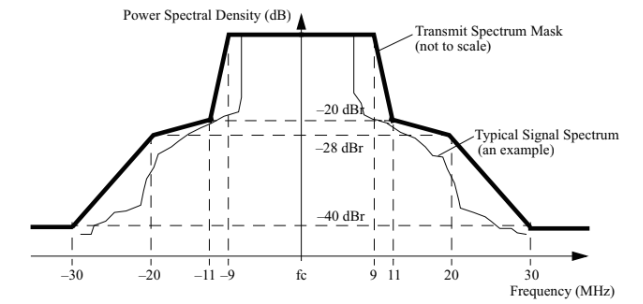
Figure 1. Transmitted spectral masks of OFDM modulation used in the IEEE 802.11 group of standards. [1]
The authors in [1] define this parameter as the I-factor and provide the normalized results. The I-factor has a cumulative effect, so the term equivalent number of users per channel should be used to calculate channel quality:

where C is the set of IEEE 802.11 channels, and N(j) is the number of users on a particular channel.
Authors in [2] are proposing the following formula for relationship between data rate and channel energetic characteristics based on Shannon’s formula (for user u):

where B is the bandwidth and SINRu is the Signal-to-interference-plus-noise ratio for the user u, that can be described as:

where  is the access point (AP), W is the set of all visible APs, v is the interfering device, P(\) are the powers,
  is the environment coefficient (from 2 to 4), N is the additive noise,
  is the coefficient of the influence of one channel to another, d(*)* is the distance in meters.
Then the scaled ACI I-factor is provided:

If the RSSI value is known and the model, that is connecting RSSI with the distance, is selected, the distance can be easily obtained. For example, if we use the classical “One-slope” model [3-5], the distance can be derived as:

where  is the reference power on the reference distance (1 m).
Nice? I think so. Even if it's just an approximation.
1.2. CCI: co-channel interference
However, the CCI case is inherently not a case of electromagnetic interference ("Sceletor will return next week with more disturbing facts").
Yes, from the point of view of physics it's the same as ACI. But now we should remember about CSMA/CA (Carrier Sense Multiple Access / Collisions Avoidence) in Wi-Fi. From the point of view of multipple acess the devices only compete for the environment, waiting for a free time slot. Devices operating on the same channel can reserve the environment for a certain period of time using NAV (Network Allocation Vector), which is a field in the transmitted frame that records the time reserved by a certain device (fig. 2).
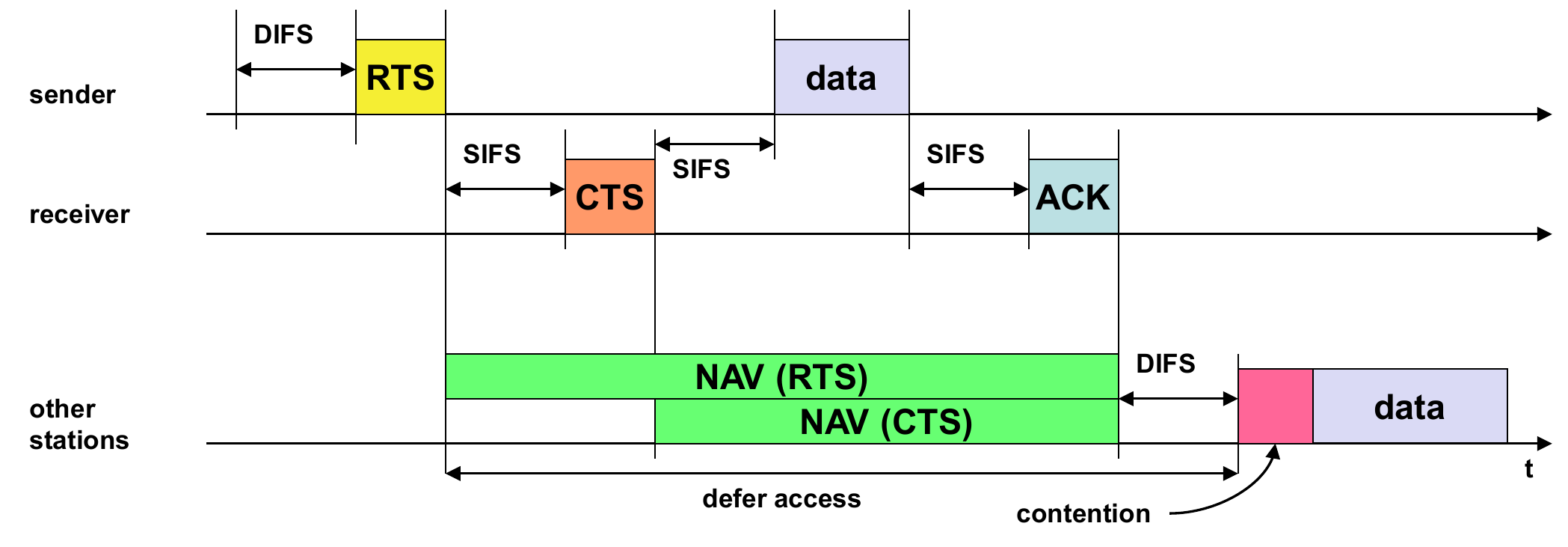
Figure 2. Scheme of environment access intervals using NAV: the station sends the RTS (request to send), the receiver responds with the CTS (clear-to-send) as a confirmation; the rest of the stations fill in their NAV, that corresponds to the required time for sending service-based and personal data.
Therefore, CCI is a more controllable case. That is why less collisions should be in CCI (remeber classical suggestion for Wi-Fi planning: 1, 6, 11 non-overlapping channels).
Thus, this case of interference should be researched separately and with including non-electromagnetic issues.
2. MatLab simulation: word "model" means world to me
The first step of the CCI case research was the simulation of the data transmission over the IEEE 802.11n standard in the WLAN toolbox of MatLab.
For this, the example [6] was used as the reference. Four cases were simulated: single Wi-Fi router (transmitter node) with one associated device (receiver node) (no interference); two, four (fig. 3) and eight simultaneously working Wi-Fi routers (interference cases).

Figure 3. The simulation of four rooms (each of them: 5 m x 5 m x 3 m) with Wi-Fi routers (red nodes) and their associated devices (blue nodes) (see Case 3 in the Table 1).
All the transmitters were configured as follows:
- MCS (modulation and coding scheme) index: 7;
- Bandwidth: 20 MHz;
- Channel: 6 (2.4 GHz);
- Guard interval: 0.8 microseconds.
The results of the simulation are provided in the Table 1.
Table 1. Matlab Simulation results
| # | Case | Throughputs (Mbps) | |
|---|---|---|---|
| 1 | Single Wi-Fi router (Node 1) and its associated device (Node 2) |
Node 1 — Node 2: 60 | |
| 2 | Two Wi-Fi routers | Node 1 — Node 3: 35.5 Node 2 — Node 4: 30.7 |
|
| 3 | Four Wi-Fi routers (fig. 3) | Node 1 — Node 5: 15.8 Node 2 — Node 6: 27.4 Node 3 — Node 7: 11.5 Node 4 — Node 8: 11.5 |
|
| 4 | Eight Wi-Fi routers | Node 1 — Node 9: 15.4 Node 2 — Node 10: 15.4 Node 3 — Node 11: 7.7 Node 4 — Node 12: 0.5 Node 5 — Node 13: 0 Node 6 — Node 14: 3.8 Node 7 — Node 15: 7.7 Node 8 — Node 16: 7.7 |
Paragraph conclusions
- First, it can be noted that the total throughput remains at the level of 60 — 65 Mbps in all cases.
- Second, the throughput is distributed unevently, some nodes can suffer from interference more than others, which illustrates the competitive nature of resource sharing.
This simulation set is used by us as the basis for the CCI case.
3. Experimental part: Try it and you shall see
Ok, if we suppose that time-frequecy resource will be shared more or less fairly let's try to obtain this in practice.
Let's do a "dirty" experiment aimed at a real life case with extremal conditions: several routers are working simultansently and trying to communicate with their stations as much as possible (imagine that all your neighboures and you want to watch 4K video streaming or play online games in the same time).
The main goals of the experimental part included:
- first, to check the theoretical assumption that the CCI channel is the worst case (formula 1), and
- second, to check how channel resources are shared between several APs.
3.1 Testbed
The tested cases included 1, 2, 3, 4, 5, 6 and 7 simultaneously working APs (access points):
- MikroTik RB951G-2HND (MIMO is supported);
- two TP-Link TL-WR740N;
- two TP-Link TL-WR741N (MIMO is supported);
- TP-Link TL-WR841N;
- TP-Link Archer C7 (MIMO is supported).
Station’s (STA) hardware and software included:
- Raspberry Pi 4 Model B with Raspbian Buster;
- D-Link DWA-160 (MIMO 2x2 is supported);
- Iperf3 program (server mode).
The scheme of the described above stand is presented in the Figure 4.

Figure 4. The scheme of the research stand.
All devices were placed in the same office room, the RSSI between APs was about -46 dBm (fig. 5), bandwidths were switched to 20 MHz. MikroTik RB951G-2HND was considered as the device under the test (DUT). Measurements were done between 9 PM and 6 AM to avoid interference from the other devices in the office building. Any produced by not Wi-Fi devices distortions (e.g. cellular networks, Bluetooth devices, microwave oven) are considered as background noise which always impacts connection quality in the case of urban indoor (either home or office).

Figure 5. The view of the stand with four simultaneously working APs.
The main advantage of the approach described above is that the heterogeneity of the devices included in the test stand allows us to conclude that the approximation was made using the model that was as close to reality as possible. The main disadvantage of this approach is that the results depend on a specific set of devices.
In addition, software channel change (from 13th to 8th) for all routers was used for the following research stand configurations to investigate the ACI case:
- 2 simultaneously working APs (MikroTik RB951G-2HND and TP-Link TL-WR741N) — the simplest case;
- 6 simultaneously working APs (MikroTik RB951G-2HND, TP-Link TL-WR841N, two TP-Link TL-WR741N, TP-Link TL-WR740N) — the most complex centra-symmetric case.
Devices that support MIMO configuration have generally reported bit rates of around 78 Mbps with a 15 MCS (Modulation and Coding Scheme) index when tested separately (without neighbors); non-MIMO devices reported about 38 Mbps with an MCS index of 7.
3.2. Results
I remind you that this is a "dirty", (pseudo)real crash test of the theory. Please, don't treat the results as kind of generalization attempt.
The case of occupying the same channel (co-channel) was as expected (2) the worst case (for two APs). In practice, this is not true (fig. 6), which may be due to the fact that CCI is not a case of electromagnetic interference and is determined by the internal multiple access mechanism of the IEEE 802.11 standards group.

Figure 6. The summarized data rate of the device under the test (DUT) and interfering devices.
Secondly, the non-linear relation between the number of devices per channel and overall data rate decreasing has been obtained (fig. 7).

Figure 7. The results of the data rates measurements (CCI case).
Confusing disproportions between consumption of resources by different devices may be explained via the variable nature of the contention window (fig. 2).
Therefore, different models can use different contention scheduling algorithms, which can produce the non-linear character of the resource's distribution.
The results of the ACI investigation (6 routers) are shown in table 2.
Table 2. Results of the ACI measurements.
| AP | Channel | Median bitrate (Mbps) | ||
|---|---|---|---|---|
| The best case (sum of median bit rates: 64.4 Mbps) |
||||
| MikroTik RB951G-2HND | 13 | 0.1 | ||
| TP-Link TL-WR741N | 13 | 0.7 | ||
| TP-Link TL-WR741N | 13 | 0.2 | ||
| TP-Link TL-WR740N | 13 | 0.1 | ||
| TP-Link TL-WR841N | 8 | 30.3 | ||
| TP-Link Archer C7 | 8 | 33.0 | ||
| The best case with symmetric channel distribution (sum of median bit rates: 55.8 Mbps) |
||||
| MikroTik RB951G-2HND | 13 | 0.1 | ||
| TP-Link TL-WR741N | 13 | 0.6 | ||
| TP-Link TL-WR741N | 13 | 1 | ||
| TP-Link TL-WR740N | 8 | 8.9 | ||
| TP-Link TL-WR841N | 8 | 18.8 | ||
| TP-Link Archer C7 | 8 | 27.0 |
Note, the best case is not symmetric (13-13-13-13-8-8), but in symmetric case (13-13-13-8-8-8) the distribution of the resources is fairer.
Paragraph conclusions
- CCI case is more complicated that it might seem;
- ACI too;
- resource allocation can depend on certain divice design (tab 2).
4. RSSI between devices: distance is matter
Ok, I agree that Wi-Fi communication of several routers in the room is more specific than realistic. Therefore, the next point is the impact of the different RSSI (Received Signal Strength Index) values between neighboring devices on the date rates.
NOTE: Here RSSI means RSSI between two Wi-Fi routers, not between a Wi-Fi router and its station. Therefore with a smaller RSSI we expect less interference and therefore a higher data rate.
4.1. Urban indoor
The first experiments in the same office showned that the data rate increases if the RSSI values decrease (fig. 8).

Figure 8. The results of the data rate measurements (MikroTik RB951G-2HND (DUT) and TP-Link TL-WR741N)
However, the CCI case did not show the dramatic difference between the summary data rates (fig. 9).

Figure 9. The results of the data rates measurements (MikroTik RB951G-2HND (DUT) and TP-Link TL-WR741N) only in case of CCI.
The explanation for the different rates and the lack of growth as RSSI decreases between APs in the case of -46 and -62 dBm may be the difference in the environment (office equipment around, overlapping walls, etc.), that affects the multipath propagation of radio waves. Simply pit, the difference in speed is more due to the environment than the RSSI between APs.
4.2. Sub-urban outdoor
Additional open-air measurements were done to avoid the impact of indoor electromagnetic wave propagation issues (fig. 10).

Figure 10. The photos of the equipment prepaired for measurements.
Two TP-Link TL-WR740N were used as APs, two Raspberry Pi 4 Model B with Raspbian Buster were used as iperf3 servers, two MacBooks Pro (16-inch, 2019) as stations with iperf3 clients (fig. 11).

Figure 11. The scheme of the second research stand.
The measurement results are presented in table 3.
Table 3. Results of the open-air set of measurements.
| RSSI between APs (dBm) | Bit rate (Mbps) TP-Link 740N |
Bit rate (Mbps) TP-Link 740N |
|||
|---|---|---|---|---|---|
| Sum. bit rate (Mbps) Without interference |
|||||
| 44 | 27,4 | 71,4 | |||
| Channels: 13 and 13 (CCI) | |||||
| -46 | 27,5 | 10,2 | 37,7 | ||
| -65 | 32,6 | 13,1 | 45,7 | ||
| -76 | 30,8 | 14,1 | 44,9 | ||
| -80 | 35,1 | 16 | 51,1 | ||
| -90 | 42,4 | 20,5 | 62,9 | ||
| Channels: 13 and 12 (ACI) | |||||
| -46 | 9,8 | 15,1 | 24,9 | ||
| -65 | 38,4 | 19,1 | 57,5 | ||
| -76 | 32,1 | 25 | 57,1 | ||
| -80 | 38,5 | 25,9 | 64,4 | ||
| -90 | 44,2 | 26,9 | 71,1 | ||
| Channels: 13 and 9 (ACI) | |||||
| -46 | 13,6 | 22 | 35,6 | ||
| -65 | 39,4 | 23,1 | 62,5 | ||
| -76 | 35,8 | 26,5 | 62,3 | ||
| -80 | 40,2 | 25,9 | 66,1 | ||
| -90 | 43,8 | 26,5 | 70,3 |
The visualization of the results shown in table 1 is presented in Figure 12.

Figure 12. The results of the second set of measurements.
This set of measurements shows that RSSI can also influence bit rate in the CCI case. Although CCI is not kind of electromagnetic interference and therefore should appear every time when the carrier sense threshold (typically -95 dBm) is crossed, the different values of RSSI may produce different probabilities of the carrier sense detection that can be reflected in the data rates.
Paragraph conclusions
- Yes, environment is (obviously) matter;
- yes, RSSI is matter and formula (5) more usefull than formula (1);
- realistic relationship between RSSI and interference is required.
5. Examples of implementation: baptism of fire
The investigated theoretical basics and collected heuristics were used by us as the basis for mass Wi-Fi optimization algorithms: changing the channel according to knowledge about what channels are occupied by neighboring devices and what the RSSI values between them (fig. 13).

Figure 13. An example of Wi-Fi spectrum visualization with the mapping with a special metric (channel quality) characterizing the interference picture in each channel.
These algorithms were used by us in several proof-of-concept (PoC) projects. The CWMP (TR-069) protocol was used as a source of information about RSSI and occupied channels. The following sections or their replacements are required:
Device.WiFi.Radio.{i}. (information about Wi-Fi radar):
- Channel (the current radio channel used by the connection);
- CurrentOperatingChannelBandwidth (the channel bandwidth currently in use (20MHz, 40MHz, 80MHz or 160MHz));
- PossibleChannels (possible radio channels for the wireless standard (a, b, g, n) and the regulatory domain);
Device.WiFi.NeighboringWiFiDiagnostic. (information about neighbors of Wi-Fi radar):
- Channel (the current radio channel used by the neighboring WiFi radio);
- SignalStrength (an indicator of radio signal strength (RSSI) of the neighboring WiFi radio measured in dBm, as an average of the last 100 packets received);
- OperatingChannelBandwidth (indicates the bandwidth at which the channel is operating).
The parameters mentioned above are also available for TR-181 model of USP (TR-369) protocol.
Moreover, obtained results were used by us in our cluster optimization framework. Cluster is a group of managed Wi-Fi routers whose connectivity can be viewed as an incomplete bipartite graph (fig. 14).

Figure 14. The example of Wi-Fi devices cluster on the city map (little bit blurred, yes).
It has been investigated, that these structures are more or less stable, however may change due to dinamically changing wireless environment (fig. 15).

Figure 15. Change in size of one selected cluster within three months (the increase in size can probably be explained by turning on/off some devices that can connect two sub-clusters).
One of the metrics for evaluation the performance of Wi-Fi optimization algorithms was the calculated derivative of traffic on devices: the difference in the number of bits collected by CWMP in two neighboring timeslots divided by the number of seconds between these timeslots (Mbps) (fig. 16). Considering this metric, we should take into account that users behave differently: someone may not use 2.4 GHz or Wi-Fi at all for some time and only service traffic will be taken into account in statistics, someone downloads only per hour peak, someone — then all day. Also, uneven use can be characteristic for different days of the week, holidays, etc. All this statistically adds up to such seemingly small IEEE 802.11n values.

Figure 16. The curve of the calculated traffic derivative (quantile 0.99 for all of the considered devices) in one of the PoC projects.
Optimization procedures were launched on November 10, 2021 for about 25 thousand devices.
The increase in traffic can be estimated at about 10%. I don't think it is an accident (I hope). Additionally, considered devices have been switched to 20 MHz operating bandwidths to avoid overlapping in overcrowded spectrum cases (18.10.2021). An increase in the traffic derivative, in this case, may correspond to the prospect of bandwidth limitation in the 2.4 GHz Wi-Fi spectrum.
Yes, it may look less impressive than some expect. However, the diamond is small, but valuable.
Conclusions and discussion
- The obtained results allow to consider the theoretical expectations regarding the distribution of recourses between IEEE 802.11 devices only as idealized abstraction.
- The resulting heuristics looks promissing, but does not guarantee incredible results.
In fact, the last conclusion is also depend on lack of required information in received data: we don't know real activity on the neighboring Wi-Fi routers. Yes, some neighbor can occupate channel, but if there is no communication with its stations we can consider this router as silent. And vice versa.
The channel utilization for neighbores will be available in modern versions of TR-181 model:
- Device.WiFi.DataElements.Network.Device.{i}.Radio.{i}.ScanResult.{i}.OpClassScan.{i}.ChannelScan.{i}.NeighborBSS.{i}.ChannelUtilization: The channel utilization reported by the neighboring BSS per the BSS Load element if present in Beacon or Probe Response frames, as defined by Section 9.4.2.28 in [802.11-2016].
So, still waiting for devices with this functionality to test our suggestions...
Moreover, the evolution of Wi-Fi standards already brings new challenges:
- The channel bonding mechanism should be considered more precisely in the case of using the 5 GHz spectrum, since bandwidth limitations can not be used at all (typical channel width is 80 MHz in urban areas).
Moreover, there are no overlapping 20 MHz channels in the 5 GHz band. Therefore, the diffecent approach should be used to calculate the I-factor [7]. - Other correlations between the number of devices occupying a channel and the level of interference can also occur in the case of IEEE 802.11ax due to the basic service set (BSS) coloring feature of the IEEE 802.11ax [8].
Perhaps, the analysis of the amount of collected data using machine learning and deep learning tools [9] can provide some solutions for optimization — we'll see.
I'll appreciate your suggestions and comments! Thanks for reading!
References
- Mi, P. and Wang, X., 2012, June. Improved channel assignment for WLANs by exploiting partially overlapped channels with novel CIR-based user number estimation. In 2012 IEEE International Conference on Communications (ICC) (pp. 6591-6595). IEEE.
- Zhou, Kunxiao, et al. "Channel assignment for WLAN by considering overlapping channels in SINR interference model." 2012 International Conference on Computing, Networking and Communications (ICNC). IEEE, 2012.
- Xue W. et al. Improved Wi-Fi RSSI measurement for indoor localization //IEEE Sensors Journal. – 2017. – Т. 17. – No. 7. – С. 2224-2230.
- Nindito S. Analisa pathloss exponent pada daerah urban dan suburban //EEPIS Final Project. – 2011.
- Li G. et al. Indoor positioning algorithm based on the improved RSSI distance model //Sensors. – 2018. – Т. 18. – No. 9. – С. 2820.
ch.mathworks.com. (n.d.). - “802.11ax Multinode System-Level Simulation of Residential Scenario Using MATLAB — MATLAB & Simulink — MathWorks Switzerland.” Ch.mathworks.com, ch.mathworks.com/help/wlan/ug/802-11ax-multinode-system-level-simulation-of-residential-scenario-using-matlab.html.
- Zankiewicz, Andrzej. "Experimental analysis of susceptibility of IEEE 802.11 ac Wave 1 networks to adjacent and co-channel interference." Przegląd Elektrotechniczny 94, no. 2 (2018): 88-91.
- A. Valkanis, A. Iossifides, P. Chatzimisios, M. Angelopoulos and V. Katos, "IEEE 802.11ax Spatial Reuse Improvement: An Interference-Based Channel-Access Algorithm," in IEEE Vehicular Technology Magazine, vol. 14, no. 2, pp. 78-84, June 2019, doi: 10.1109/MVT.2019.2904101.
- Jeunen, O., Bosch, P., Van Herwegen, M., Van Doorselaer, K., Godman, N. and Latré, S., 2018, November. A machine learning approach for IEEE 802.11 channel allocation. In 2018 14th International Conference on Network and Service Management (CNSM) (pp. 28-36). IEEE.
Acknowledgments
Thanks to my colleagues Marat Azizov, Rauf Agishev, Ivan Antonyuk, Roman Kirillov, Danil Ibragimov, Alexander Avdonin and Rail Yakupov for their suggestions, and advice and help with experiments! Thanks a lot to my colleagues Vladislav Sadretdinov and Linar Minkhaerov for their work on UI in PoCs projects! Special thanks to Sergey Filimonov for his corrections of the text (unfortunately, my English is not perfect)!
P.S.
This will be titled as "The issues of the calculation of IEEE 802.11n co-channel interference (CCI) and adjacent channel interference (ACI) coefficients based on available in CWMP (TR-069) and USP (TR-369) protocols parameters" if this will be a scientific article, I think.
