Queries in PostgreSQL. Sequential scan
In previous articles we discussed how the system plans a query execution and how it collects statistics to select the best plan. The following articles, starting with this one, will focus on what a plan actually is, what it consists of, and how it is executed.
In this article, I will demonstrate how the planner calculates execution costs. I will also discuss access methods and how they affect these costs, and use the sequential scan method as an illustration. Lastly, I will talk about parallel execution in PostgreSQL, how it works, and when to use it.
I will use several seemingly complicated math formulas later in the article. You don't have to memorize any of them to get to the bottom of how the planner works; they are merely there to show where I get my numbers from.
Pluggable storage engines
The PostgreSQL approach to storing data on disk will not be optimal for every possible type of load. Thankfully, you have options. Delivering on its promise of extensibility, PostgreSQL 12 and higher supports custom table access methods (storage engines), although it ships only with the stock one, heap:
SELECT amname, amhandler FROM pg_am WHERE amtype = 't'; amname | amhandler
−−−−−−−−+−−−−−−−−−−−−−−−−−−−−−−
heap | heap_tableam_handler
(1 row)You can specify an engine when creating a table (CREATE TABLE ... USING). If you don't, the engine defined in default_table_access_method is used.
The pg_am catalog stores engine names (amname column) as well as their handler functions (amhandler). Every storage engine comes with an interface that the core needs in order to make use of the engine. The handler function's job is to return all the necessary information about the interface structure.
The majority of storage engines make use of the existing core system components:
- Transaction manager, including ACID support and snapshot isolation.
- The buffer manager.
- I/O subsystem.
- TOAST.
- Query optimizer and executor.
- Index support.
An engine might not necessarily use all of these components, but the ability is still there.
Then, there are things that an engine must define:
- Row version format and data structure.
- Table scan routines.
- Insert, delete, update, and lock routines.
- Row version visibility rules.
- Vacuuming and analysis processes.
- Sequential scan cost estimation process.
Traditionally, PostgreSQL used a single data storage system that was built into the core directly, without an interface. This makes creating a new interface — accommodating all the long-standing particularities of the standard engine and not interfering with other access methods — a challenge and a half.
There is an issue with write-ahead logging, for example. Some access methods want to log engine-specific operations, which the core knows nothing about. The existing Generic WAL Records mechanism is rarely an option because of significant overhead costs. You could devise a separate interface for new log record types, but this makes crash recovery dependent on external code, which is something you always want to avoid. So far, rebuilding the core to fit a new engine remains the only viable option.
Speaking of new engines, there are several currently in development. Here are some of the more prominent ones:
- Zheap is an engine that tackles table bloating. It implements in-place row version update and stores snapshot data in a separate undo storage. This engine is effective for update-intensive workloads. The engine design resembles that of Oracle's, with some differences here and there (for example, the index access method interface does not support indexes with their own multiversion concurrency control).
- Zedstore implements columnar storage and is designed to handle OLAP transactions more efficiently. It organizes data into a primary B-tree of row version IDs, and each column is stored in its own B-tree, which references the primary one. In the future, the engine may support storing multiple columns inside one tree, essentially becoming a hybrid storage engine.
Sequential scan
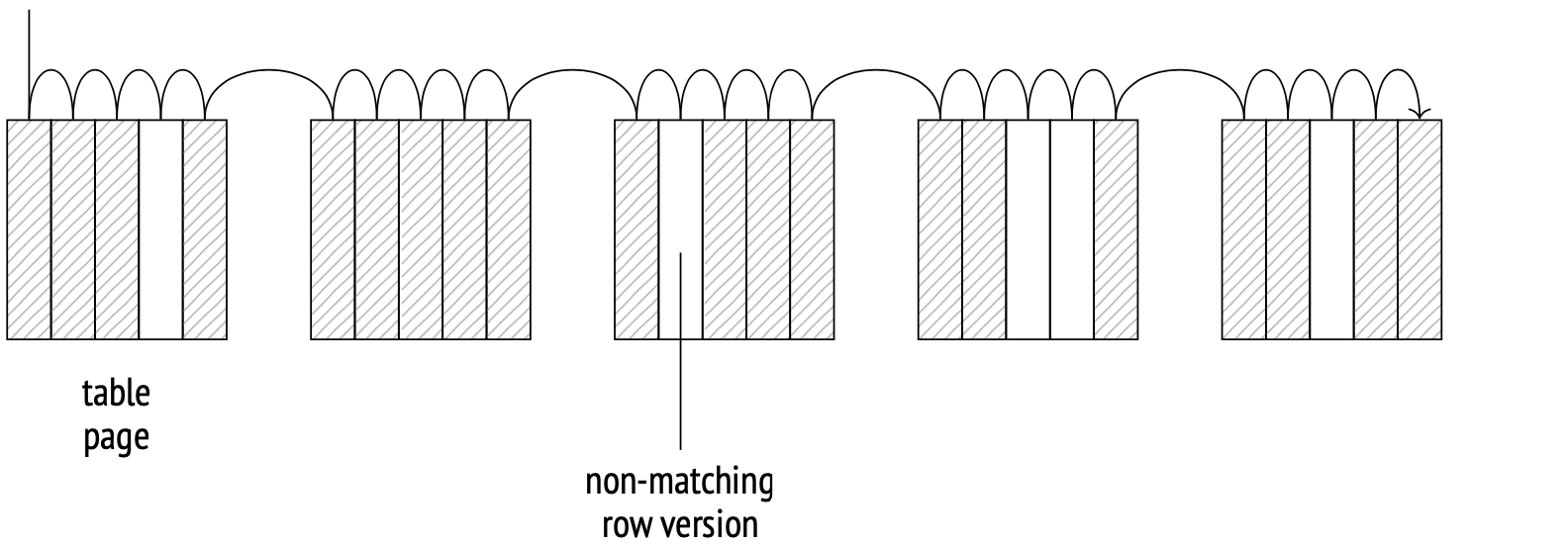
The storage engine determines how table data is physically distributed on disk and provides a method to access it. Sequential scan is a method that scans the file (files) of the main table fork entirely. On each page, the system checks the visibility of each row version, and also discards the versions that don't match the query.
The scanning is done through the buffer cache. The system uses a small buffer ring to prevent larger tables from pushing potentially useful data from the cache. When another process needs to scan the same table, it joins the buffer ring, saving disk read times. Therefore, scanning does not necessarily start from the beginning of the file.
Sequential scan is the most cost-effective way of scanning a whole table or a significant portion of it. In other words, sequential scan is efficient when selectivity is low. At higher selectivity, when only a small fraction of rows in a table meets the filter requirements, it's usually better to use index scan.
Example plan
A sequential scan stage in an execution plan is represented with a Seq Scan node.
EXPLAIN SELECT * FROM flights; QUERY PLAN
−−−−−−−−−−−−−−−−−−−−−−−−−−−−−−−−−−−−−−−−−−−−−−−−−−−−−−−−−−−−−−−−
Seq Scan on flights (cost=0.00..4772.67 rows=214867 width=63)
(1 row)Row count estimate is a basic statistic:
SELECT reltuples FROM pg_class WHERE relname = 'flights'; reltuples
−−−−−−−−−−−
214867
(1 row)When estimating costs, the optimizer takes into account disk input/output and CPU processing costs.
The I/O cost is estimated as a single page fetch cost multiplied by the number of pages in a table, provided that the pages are fetched sequentially. When the buffer manager requests a page from the operating system, the system actually reads a larger chunk of data from disk, so the next several pages will probably be in the operating system's cache already. This makes the sequential fetch cost (which the planner weights at seq_page_cost, 1 by default) considerably lower than the random access fetch cost (which is weighted at random_page_cost, 4 by default).
The default weights are appropriate for HDD drives. If you are using SSDs, the random_page_cost can be set significantly lower (seq_page_cost is usually left at 1 as the reference value). The costs depend on hardware, so they are usually set at the tablespace level (ALTER TABLESPACE ... SET).
SELECT relpages, current_setting('seq_page_cost') AS seq_page_cost,
  relpages * current_setting('seq_page_cost')::real AS total
FROM pg_class WHERE relname='flights';
relpages | seq_page_cost | total
−−−−−−−−−−+−−−−−−−−−−−−−−−+−−−−−−−
2624 | 1 | 2624
(1 row)This formula perfectly illustrates the result of table bloating due to late vacuuming. The larger the main table fork, the more pages there are to fetch, regardless of whether the data in these pages is up-to-date or not.
The CPU processing cost is estimated as the sum of processing costs for each row version (weighted by the planner at cpu_tuple_cost, 0.01 by default):
SELECT reltuples,
  current_setting('cpu_tuple_cost') AS cpu_tuple_cost,
  reltuples * current_setting('cpu_tuple_cost')::real AS total
FROM pg_class WHERE relname='flights';
 reltuples | cpu_tuple_cost | total
−−−−−−−−−−−+−−−−−−−−−−−−−−−−+−−−−−−−−−
    214867 |           0.01 | 2148.67
(1 row)
The sum of the two costs is the total plan cost. The plan's startup cost is zero because sequential scan does not require any preparation steps.
Any table filters will be listed in the plan below the Seq Scan node. The row count estimate will take into account the selectivity of filters, and the cost estimate will include their processing costs. The EXPLAIN ANALYZE command displays both the actual number of scanned rows and the number of rows removed by the filters:
EXPLAIN (analyze, timing off, summary off)
SELECT * FROM flights WHERE status = 'Scheduled';
QUERY PLAN
−−−−−−−−−−−−−−−−−−−−−−−−−−−−−−−−−−−−−−−−−−−−−−−−
Seq Scan on flights
(cost=0.00..5309.84 rows=15383 width=63)
(actual rows=15383 loops=1)
Filter: ((status)::text = 'Scheduled'::text)
Rows Removed by Filter: 199484
(5 rows)Example plan with aggregation
Consider this execution plan that involves aggregation:
EXPLAIN SELECT count(*) FROM seats; QUERY PLAN
−−−−−−−−−−−−−−−−−−−−−−−−−−−−−−−−−−−−−−−−−−−−−−−−−−−−−−−−−−−−−−
Aggregate (cost=24.74..24.75 rows=1 width=8)
−> Seq Scan on seats (cost=0.00..21.39 rows=1339 width=0)
(2 rows)There are two nodes in this plan: Aggregate and Seq Scan. Seq Scan scans the table and passes the data up to Aggregate, while Aggregate counts the rows on an ongoing basis.
Notice that the Aggregate node has a startup cost: the cost of aggregation itself, which needs all the rows from the child node to compute. The estimate is calculated based on the number of input rows multiplied by the cost of an arbitrary operation (cpu_operator_cost, 0.0025 by default):
SELECT
  reltuples,
  current_setting('cpu_operator_cost') AS cpu_operator_cost,
  round((
    reltuples * current_setting('cpu_operator_cost')::real
  )::numeric, 2) AS cpu_cost
FROM pg_class WHERE relname='seats';
reltuples | cpu_operator_cost | cpu_cost
−−−−−−−−−−−+−−−−−−−−−−−−−−−−−−−+−−−−−−−−−−
1339 | 0.0025 | 3.35
(1 row)The estimate is then added to the Seq Scan node's total cost.
The Aggregate's total cost is then increased by cpu_tuple_cost, which is the processing cost of the resulting output row:
WITH t(cpu_cost) AS (
  SELECT round((
    reltuples * current_setting('cpu_operator_cost')::real
  )::numeric, 2)
  FROM pg_class WHERE relname = 'seats'
)
SELECT 21.39 + t.cpu_cost AS startup_cost,
  round((
    21.39 + t.cpu_cost +
    1 * current_setting('cpu_tuple_cost')::real
  )::numeric, 2) AS total_cost
FROM t;
startup_cost | total_cost
−−−−−−−−−−−−−−+−−−−−−−−−−−−
24.74 | 24.75
(1 row)Parallel execution plans
In PostgreSQL 9.6 and higher, parallel execution of plans is a thing. Here's how it works: the leader process creates (via postmaster) several worker processes. These processes then simultaneously execute a section of the plan in parallel. The results are then gathered at the Gather node by the leader process. While not occupied with gathering data, the leader process may participate in the parallel calculations as well.
You can disable this behavior by setting the parallel_leader_participation parameter to 0, but only in version 11 or higher.

Spawning new processes and sending data between them add to the total cost, so you may often be better off not using parallel execution at all.
Besides, there are operations that simply can't be executed in parallel. Even with the parallel mode enabled, the leader process will still execute some of the steps alone, sequentially.
Parallel sequential scan
The method's name might sound controversial, claiming to be parallel and sequential at the same time, but that's exactly what's going on at the Parallel Seq Scan node. From the disk's point of view, all file pages are fetched sequentially, same as they would be with a regular sequential scan. The fetching, however, is done by several processes working in parallel. The processes synchronize their fetching schedule in a special shared memory section in order to avoid fetching the same page twice.
The operating system, on the other hand, does not recognize this fetching as sequential. From its perspective, it's just several processes requesting seemingly random pages. This breaks prefetching that serves us so well with regular sequential scan. The issue was fixed in PostgreSQL 14, when the system started assigning each parallel process several sequential pages to fetch at once instead of just one.
Parallel scanning by itself doesn't help much with cost efficiency. In fact, all it does is add the cost of data transfers between processes on top of the regular page fetch cost. However, if the worker processes not only scan the rows, but also process them to some extent (for example, aggregate), then you may save a lot of time.
Example parallel plan with aggregation
The optimizer sees this simple query with aggregation on a large table and decides that the optimal strategy is the parallel mode:
EXPLAIN SELECT count(*) FROM bookings; QUERY PLAN
−−−−−−−−−−−−−−−−−−−−−−−−−−−−−−−−−−−−−−−−−−−−−−−−−−−−−−−−−−−−−−
Finalize Aggregate (cost=25442.58..25442.59 rows=1 width=8)
−> Gather (cost=25442.36..25442.57 rows=2 width=8)
Workers Planned: 2
−> Partial Aggregate
(cost=24442.36..24442.37 rows=1 width=8)
−> Parallel Seq Scan on bookings
(cost=0.00..22243.29 rows=879629 width=0)
(7 rows)All the nodes below Gather are the parallel section of the plan. It will be executed by all worker processes (2 of them are planned in this case) and the leader process (unless disabled by the parallel_leader_participation option). The Gather node and all the nodes above it are executed sequentially by the leader process.
Consider the Parallel Seq Scan node, where the scanning itself happens. The rows field shows an estimate of rows to be processed by one process. There are two worker processes planned, and the leader process will assist too, so the rows estimate equals the total table row count divided by 2.4 (2 for the worker processes and 0.4 for the leader; the more there are workers, the less the leader contributes).
SELECT reltuples::numeric, round(reltuples / 2.4) AS per_process
FROM pg_class WHERE relname = 'bookings';
reltuples | per_process
−−−−−−−−−−−+−−−−−−−−−−−−−
2111110 | 879629
(1 row)Parallel Seq Scan cost is calculated in mostly the same way as Seq Scan cost. We win time by having each process handle fewer rows, but we still read the table through-and-through, so the I/O cost isn't affected:
SELECT round((
  relpages * current_setting('seq_page_cost')::real +
  reltuples / 2.4 * current_setting('cpu_tuple_cost')::real
)::numeric, 2)
FROM pg_class WHERE relname = 'bookings';
round
−−−−−−−−−−
22243.29
(1 row)The Partial Aggregate node aggregates all the data produced by the worker process (counts the rows, in this case).
The aggregate cost is calculated in the same way as before and added to the scan cost.
WITH t(startup_cost) AS (
  SELECT 22243.29 + round((
    reltuples / 2.4 * current_setting('cpu_operator_cost')::real
  )::numeric, 2)
  FROM pg_class WHERE relname='bookings'
)
SELECT startup_cost,
  startup_cost + round((
    1 * current_setting('cpu_tuple_cost')::real
  )::numeric, 2) AS total_cost
FROM t;
startup_cost | total_cost
−−−−−−−−−−−−−−+−−−−−−−−−−−−
24442.36 | 24442.37
(1 row)The next node, Gather, is executed by the leader process. This node starts worker processes and gathers their output data.
The cost of starting up a worker process (or several; the cost doesn't change) is defined by the parameter parallel_setup_cost (1000 by default). The cost of sending a single row from one process to another is set by parallel_tuple_cost (0.1 by default). The bulk of the node cost is the initialization of the parallel processes. It is added to the Partial Aggregate node startup cost. There is also the transmission of two rows; this cost is added to the Partial Aggregate node's total cost.
SELECT
24442.36 + round(
  current_setting('parallel_setup_cost')::numeric,
2) AS setup_cost,
24442.37 + round(
  current_setting('parallel_setup_cost')::numeric +
  2 * current_setting('parallel_tuple_cost')::numeric,
2) AS total_cost;
setup_cost | total_cost
−−−−−−−−−−−−+−−−−−−−−−−−−
25442.36 | 25442.57
(1 row)The Finalize Aggregate node joins together the partial data collected by the Gather node. Its cost is assessed just like with a regular Aggregate. The startup cost comprises the aggregation cost of three rows and the Gather node total cost (because Finalize Aggregate needs all its output to compute). The cherry on top of the total cost is the output cost of one resulting row.
WITH t(startup_cost) AS (
  SELECT 25442.57 + round((
    3 * current_setting('cpu_operator_cost')::real
  )::numeric, 2)
  FROM pg_class WHERE relname = 'bookings'
)
SELECT startup_cost,
  startup_cost + round((
    1 * current_setting('cpu_tuple_cost')::real
  )::numeric, 2) AS total_cost
FROM t;
startup_cost | total_cost
−−−−−−−−−−−−−−+−−−−−−−−−−−−
25442.58 | 25442.59
(1 row)Parallel processing limitations
There are several limitations to parallel processing that should be kept in mind.
Number of worker processes
The use of background worker processes is not limited to parallel query execution: they are used by the logical replication mechanism and may be created by extensions. The system can simultaneously run up to max_worker_processes background workers (8 by default).
Out of those, up to max_parallel_workers (also 8 by default) can be assigned to parallel query execution.
The number of allowed worker processes per leader process is set by max_parallel_workers_per_gather (2 by default).
You may choose to change these values based on several factors:
- Hardware configuration: the system must have spare processor cores.
- Table sizes: parallel queries are helpful with larger tables.
- Load type: the queries that benefit the most from parallel execution should be prevalent.
These factors are usually true for OLAP systems and false for OLTPs.
The planner will not even consider parallel scanning unless it expects to read at least min_parallel_table_scan_size of data (8MB by default).
Below is the formula for calculating the number of planned worker processes:

In essence, every time the table size triples, the planner adds one more parallel worker. Here's an example table with the default parameters.
| Table, MB | Number of workers |
|---|---|
| 8 | 1 |
| 24 | 2 |
| 72 | 3 |
| 216 | 4 |
| 648 | 5 |
| 1944 | 6 |
The number of workers can be explicitly set with the table storage parameter parallel_workers.
The number of workers will still be limited by the max_parallel_workers_per_gather parameter, though.
Let's query a small 19MB table. Only one worker process will be planned and created (see Workers Planned and Workers Launched):
EXPLAIN (analyze, costs off, timing off)
SELECT count(*) FROM flights;
QUERY PLAN
−−−−−−−−−−−−−−−−−−−−−−−−−−−−−−−−−−−−−−−−−−−−−−−−−−−−−−−−−−−−−−−−−−−−−
Finalize Aggregate (actual rows=1 loops=1)
−> Gather (actual rows=2 loops=1)
Workers Planned: 1
Workers Launched: 1
−> Partial Aggregate (actual rows=1 loops=2)
−> Parallel Seq Scan on flights (actual rows=107434 lo...
(6 rows)Now let's query a 105MB table. The system will create only two workers, obeying the max_parallel_workers_per_gather limit.
EXPLAIN (analyze, costs off, timing off)
SELECT count(*) FROM bookings;
QUERY PLAN
−−−−−−−−−−−−−−−−−−−−−−−−−−−−−−−−−−−−−−−−−−−−−−−−−−−−−−−−−−−−−−−−−−−−−
Finalize Aggregate (actual rows=1 loops=1)
−> Gather (actual rows=3 loops=1)
Workers Planned: 2
Workers Launched: 2
−> Partial Aggregate (actual rows=1 loops=3)
−> Parallel Seq Scan on bookings (actual rows=703703 l...
(6 rows)If the limit is increased, three workers are created:
ALTER SYSTEM SET max_parallel_workers_per_gather = 4;
SELECT pg_reload_conf();
EXPLAIN (analyze, costs off, timing off)
SELECT count(*) FROM bookings;
QUERY PLAN
−−−−−−−−−−−−−−−−−−−−−−−−−−−−−−−−−−−−−−−−−−−−−−−−−−−−−−−−−−−−−−−−−−−−−
Finalize Aggregate (actual rows=1 loops=1)
−> Gather (actual rows=4 loops=1)
Workers Planned: 3
Workers Launched: 3
−> Partial Aggregate (actual rows=1 loops=4)
−> Parallel Seq Scan on bookings (actual rows=527778 l...
(6 rows)If there are more planned workers than available worker slots in the system when the query is executed, only the available number of workers will be created.
Non-parallelizable queries
Not every query can be parallelized. These are the types of non-parallelizable queries:
Queries that modify or lock data (
UPDATE,DELETE,SELECT FOR UPDATEetc.). In PostgreSQL 11, such queries can still execute in parallel when called within commandsCREATE TABLE AS,SELECT INTOandCREATE MATERIALIZED VIEW(and in version 14 and higher also withinREFRESH MATERIALIZED VIEW). AllINSERToperations will still execute sequentially even in these cases, however.
Any queries that can be suspended during execution. Queries inside a cursor, including those in PL/pgSQL FOR loops.
Queries that call
PARALLEL UNSAFEfunctions. By default, this includes all user-defined functions and some of the standard ones. You can get the complete list of unsafe functions from the system catalog:
SELECT * FROM pg_proc WHERE proparallel = 'u';
Queries from within functions called from within an already parallelized query (to avoid creating new background workers recursively).
Future PostgreSQL versions may remove some of these limitations. Version 12, for example, added the ability to parallelize queries at the Serializable isolation level.
There are several possible reasons why a query will not run in parallel:
- It is non-parallelizable in the first place.
- Your configuration prevents the creation of parallel plans (including when a table is smaller than the parallelization threshold).
- The parallel plan is more costly than a sequential one.
If you want to force a query to be executed in parallel — for research or other purposes — you can set the parameter force_parallel_mode on. This will make the planner always produce parallel plans, unless the query is strictly non-parallelizable:
EXPLAIN SELECT * FROM flights; QUERY PLAN
−−−−−−−−−−−−−−−−−−−−−−−−−−−−−−−−−−−−−−−−−−−−−−−−−−−−−−−−−−−−−−−−
Seq Scan on flights (cost=0.00..4772.67 rows=214867 width=63)
(1 row)SET force_parallel_mode = on;
EXPLAIN SELECT * FROM flights;QUERY PLAN
−−−−−−−−−−−−−−−−−−−−−−−−−−−−−−−−−−−−−−−−−−−−−−−−−−−−−−−−−−−−−−−−−−−−−
Gather (cost=1000.00..27259.37 rows=214867 width=63)
Workers Planned: 1
Single Copy: true
−> Seq Scan on flights (cost=0.00..4772.67 rows=214867 width=63)
(4 rows)Parallel restricted queries
In general, the benefit of parallel planning depends mostly on how much of the plan is parallel-compatible. There are, however, operations that technically do not prevent parallelization, but can only be executed sequentially and only by the leader process. In other words, these operations cannot appear in the parallel section of the plan, below Gather.
Non-expandable subqueries. A basic example of an operation containing non-expandable subqueries is a common table expression scan (the CTE Scan node below):
EXPLAIN (costs off)
WITH t AS MATERIALIZED (
  SELECT * FROM flights
)
SELECT count(*) FROM t;
QUERY PLAN
−−−−−−−−−−−−−−−−−−−−−−−−−−−−
Aggregate
CTE t
−> Seq Scan on flights
−> CTE Scan on t
(4 rows)If the common table expression is not materialized (which became possible only in PostgreSQL 12 and higher), then there is no CTE Scan node and no problem.
The expression itself can be processed in parallel, if it's the quicker option.
EXPLAIN (costs off)
WITH t AS MATERIALIZED (
  SELECT count(*) FROM flights
)
SELECT * FROM t;
QUERY PLAN
−−−−−−−−−−−−−−−−−−−−−−−−−−−−−−−−−−−−−−−−−−−−−−−−−
CTE Scan on t
CTE t
−> Finalize Aggregate
−> Gather
Workers Planned: 1
−> Partial Aggregate
−> Parallel Seq Scan on flights
(7 rows)Another example of a non-expandable subquery is a query with a SubPlan node.
EXPLAIN (costs off)
SELECT *
FROM flights f
WHERE f.scheduled_departure > ( -- SubPlan
  SELECT min(f2.scheduled_departure)
  FROM flights f2
  WHERE f2.aircraft_code = f.aircraft_code
);
QUERY PLAN
−−−−−−−−−−−−−−−−−−−−−−−−−−−−−−−−−−−−−−−−−−−−−−−−−−−−−−−
Seq Scan on flights f
Filter: (scheduled_departure > (SubPlan 1))
SubPlan 1
−> Aggregate
−> Seq Scan on flights f2
Filter: (aircraft_code = f.aircraft_code)
(6 rows)The first two rows display the plan of the main query: scan the flights table and filter each row. The filter condition includes a subquery, the plan of which follows the main plan. The SubPlan node is executed multiple times: once per scanned row, in this case.
The Seq Scan parent node cannot be parallelized because it needs the SubPlan output to proceed.
The last example is executing a non-expandable subquery represented by an InitPlan node.
EXPLAIN (costs off)
SELECT *
FROM flights f
WHERE f.scheduled_departure > ( -- SubPlan
  SELECT min(f2.scheduled_departure) FROM flights f2
  WHERE EXISTS ( -- InitPlan
    SELECT *
    FROM ticket_flights tf
    WHERE tf.flight_id = f.flight_id
  )
);
QUERY PLAN
−−−−−−−−−−−−−−−−−−−−−−−−−−−−−−−−−−−−−−−−−−−−−−−−−−−−−−−−
Seq Scan on flights f
Filter: (scheduled_departure > (SubPlan 2))
SubPlan 2
−> Finalize Aggregate
InitPlan 1 (returns $1)
−> Seq Scan on ticket_flights tf
Filter: (flight_id = f.flight_id)
−> Gather
Workers Planned: 1
Params Evaluated: $1
−> Partial Aggregate
−> Result
One−Time Filter: $1
−> Parallel Seq Scan on flights f2
(14 rows)Unlike a SubPlan, an InitPlan node executes only once (in this case, once per SubPlan 2 execution).
The InitPlan node's parent can't be parallelized, but nodes that use InitPlan output can, as illustrated here.
Temporary tables. Temporary tables can only be scanned sequentially because only the leader process has access to them.
CREATE TEMPORARY TABLE flights_tmp AS SELECT * FROM flights;
EXPLAIN (costs off)
SELECT count(*) FROM flights_tmp;
QUERY PLAN
−−−−−−−−−−−−−−−−−−−−−−−−−−−−−−
Aggregate
−> Seq Scan on flights_tmp
(2 rows)Parallel restricted functions. Calls of functions labeled as PARALLEL RESTRICTED are only allowed within the sequential part of the plan. You can find the list of the restricted functions in the system catalog:
SELECT * FROM pg_proc WHERE proparallel = 'r';Only label your own functions PARALLEL RESTRICTED (not to mention PARALLEL SAFE) after thoroughly studying the existing limitations and with great care.
To be continued.
