During the last decades, the world’s population has been developing as an information society, which means that information started to play a substantial end-to-end role in all life aspects and processes. In view of the growing demand for a free flow of information, social networks have become a force to be reckoned with. The ways of war-waging have also changed: instead of conventional weapons, governments now use political warfare, including fake news, a type of propaganda aimed at deliberate disinformation or hoaxes. And the lack of content control mechanisms makes it easy to spread any information as long as people believe in it.
Based on this premise, I’ve decided to experiment with different NLP approaches and build a classifier that could be used to detect either bots or fake content generated by trolls on Twitter in order to influence people.
In this first part of the article, I will cover the data collection process, preprocessing, feature extraction, classification itself and the evaluation of the models’ performance. In Part 2, I will dive deeper into the troll problem, conduct exploratory analysis to find patterns in the trolls’ behaviour and define the topics that seemed of great interest to them back in 2016.
Features for analysis
From all possible data to use (like hashtags, account language, tweet text, URLs, external links or references, tweet date and time), I settled upon English tweet text, Russian tweet text and hashtags. Tweet text is the main feature for analysis because it contains almost all essential characteristics that are typical for trolling activities in general, such as abuse, rudeness, external resources references, provocations and bullying. Hashtags were chosen as another source of textual information as they represent the central message of a tweet in one or two words.
Among all the other features, I also considered using a tweet’s date and time metadata because it seemed pretty handy according to various experiments. However, it turned out that there were no patterns in the data on the troll tweets I obtained.
Data collection
Having done an extensive research of the state-of-the-art techniques dealing with the troll problem, I proceeded with data collection. Data sources vary: you can either use datasets provided by Twitter itself, research and data platforms or by companies such as kaggle.com or data.world. Besides, there are some data sets freely available on github.com provided by enthusiasts. However, after some rumination, I’ve decided to use the Twitter data to avoid untrustworthy sources and irrelevant data especially taking into account that Twitter, by that time, announced that they were making publicly available archives of tweets and media that they assumed were created from potentially state-backed information operations.
For the “troll” data, I was especially interested in two datasets: the one that was potentially related to tweets from Russia and the other one dedicated to the tweets of Internet Research Agency (IRA). This agency was considered responsible for a potential state-backed campaign aimed at influencing people in the USA and, thus, affecting Presidential Elections. In particular, there were 2288 and 765,248 values in each dataset, respectively.
For the “non-troll” (user) data, I used Twitter-provided API and downloaded almost 100,000 tweets on different topics, including books, news and politics. Tweets on such topics as news and politics are supposed to be close to the topics discussed by troll accounts, and quotations from books containing conversations on the relevant topics were added to create a negative dataset with diversified discussion. I also used regular conversational tweets from verified users.
In general, the more similar positive and negative data are the more relevant results of defining ”trolls” or ”non-trolls” we receive.
Preprocessing and feature extraction
Speaking of feature extraction, a classical Bag of Words approach is still the most popular solution for this kind of work. At the same time, the Word Embeddings approach is considered more sophisticated. Usually, the classification of tweets requires a good lexicon representation. So, I compared them using TfidfVectorizer (chosen over CountVectorizer as the latter cannot process large amounts of data) for the bag-of-words model and Glove for the word embeddings one.
In terms of preprocessing, for efficient classification, in this case I needed to conduct tokenisation, normalisation, noise removal, stopword removal, lowercasing and lemmatisation (only for the word embeddings).
For lowercasing, my datasets included a lot of abbreviations, such as “US” or “U.S.”, which, if converted to “us”, could affect the experiment, so I had to think carefully before using preprocessing incorporated in the libraries providing different bag-of-words models, and conduct various experiments before picking the right model.
It is also not always recommended to use lemmatisation or stemming because it could theoretically lead to a change of initial meaning of the unigram which, in its turn, might substitute the overall result, especially taking into account that I was going to visualise different patterns of the initial tweet text. However, in reality, it turned out that lemmatisation actually works very well with the word embeddings model and leads to higher accuracy when it comes to further classification.
Another issue to ponder on was stopword removal. At first glance, it seems obvious that such words as “the”, “and” or “a” should be removed but they can be informative for future predictions when classifying the style of writing or personality (which might be the case here). In the end, however, I removed them for the word embeddings model because the advantages of such removal outweighed the possible disadvantages, which was noticeable in the final classification results.
Classification and evaluation
Based on the literature review for the classification part of the project, it was decided to use Support Vector Machine and Multinomial Naive Bayes Classifiers. They are well-recognised classifiers among data scientists as some of the best solutions for tweet data.
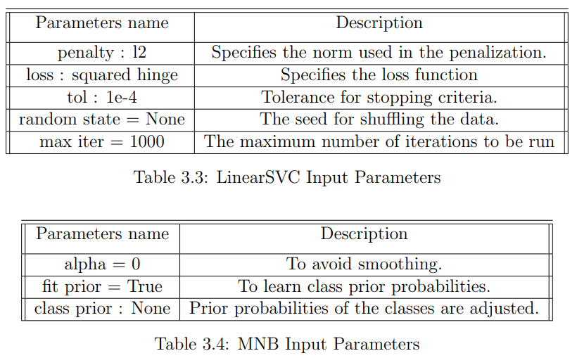
For the SVM, I was interested in C-Support Vector Classification and Linear Support Vector Classification classifiers for comparison. It turned out that the SVC classifier cannot process vast amounts of data for a reasonable amount of time while LinearSVC was pretty fast. Higher evaluation scores were also received with LinearSVC.
The Multinomial Naive Bayes classifier is considered one of the most efficient solutions for text classification with such discrete features as word counts. Thus, it works perfectly with the Bag of Words model. The multinomial distribution typically requires integer feature counts. Therefore, it was decided to include this classifier in the analyses to conduct binary classification.
SVM is the classifier that is usually trained on data belonging to one of two classes. The classifier infers the properties of ‘good’ cases and from these properties can predict which examples are unlike the common examples. Binary SVM is trained on data with both classes. The classifier predicts classes by finding the best hyperplane that separates all data points of one class of those from another class.
The Naive Bayes classifier is very efficient in supervised learning settings. Although there is not a single algorithm for training such classifiers, there is a universal principle: all Naive Bayes classifiers assume that all the features are independent of each other, based on these features classes might be predicted.

Results
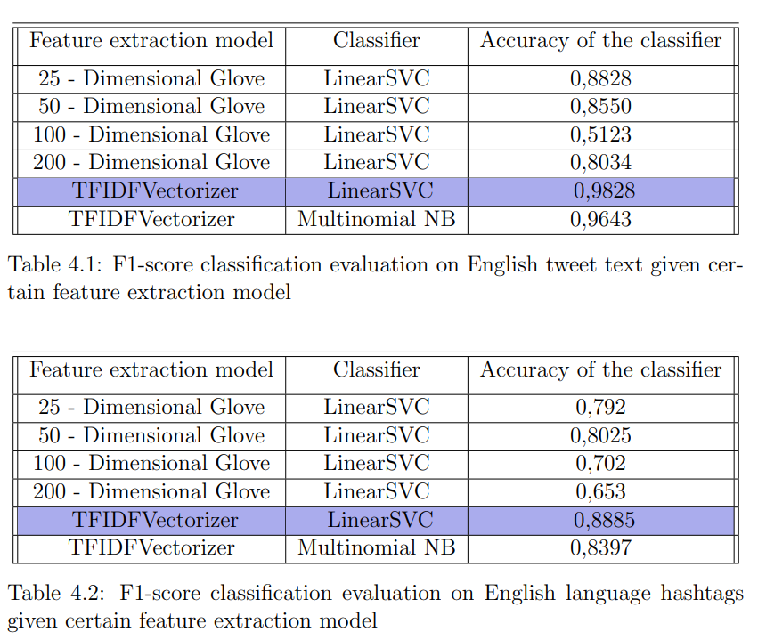
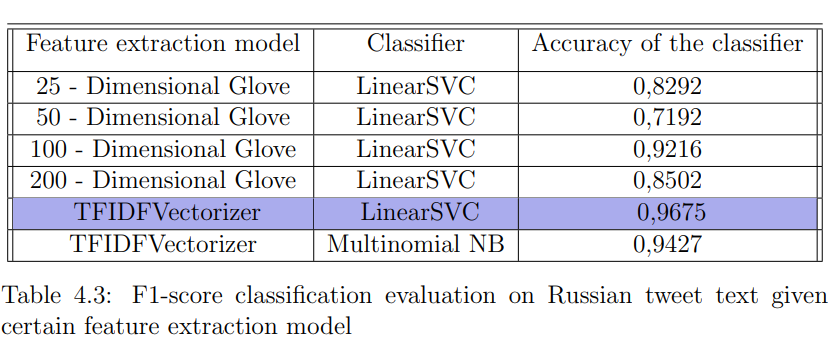
According to the results of my experiments, for all three cases (English tweet text, Russian tweet text, and hashtags), among the feature extraction models, the most significant contribution to classification was made by TFIDFVectorizer, which implied the classical Bag of Words approach. Moreover, it was the winning model for both LinearSVC and MultinomialNB classifiers, which made each of them predict more accurately than LinearSVC with all possible Glove models.


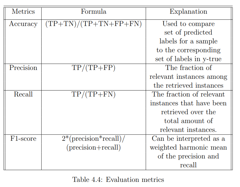
Below you can find a table with metrics I used for analysing the results of the classification where TP is the number of true positive predictions; TN is the number of true negative predictions; FP is the number of false positive predictions; and FN is the number of false negative predictions.

According to my results, the accuracy measure of LinearSVC classification performance was better than the Multinomial Naive Bayes classifier in all three cases. You can see the evaluation report and the confusion matrix for the English tweet text classification below.

Continued with EDA, topic modelling, and conclusions in Part 2 .