NickThe1 Dec 18 2022 at 12:30

Asymmetric horizontal distribution for time series

4 min

1.5K

Introduction

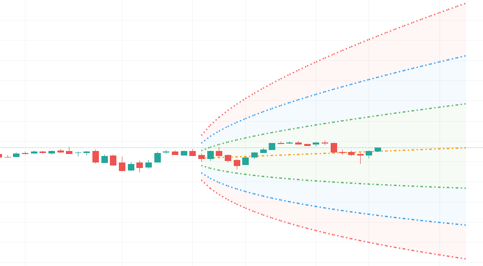
The goal of paper is to demonstrate non-trivial approaches to give statistical estimate for forecast result. Idea comes from probability cone concept. A probability cone is an indicator that forecasts a statistical distribution from a set point in time into the future. This acticle provide alternative approaches using machine learning, regression analysis.

There are properties of probability cone

Forecast a Standard or Laplace distribution.
Change the how many bars the cones will lookback and sample in their calculations.
Set how many bars to forecast the cones.
Let the cones follow price from a set number of bars back.

As we may see cone is parametric and non-robust model that takes into accout only few values. It will be solved by our methods. For accomplishing that goal, we need to collect data, preprocess it, train model, assing confidence intervals for forecast values.

Collecting data

We collected data via yfinance library and saved it to database.

start_period = "2021-01-01" end_period = "2022-01-01" interval = "1h"

def collect_save_data(assets, interval, start_period, end_period): collected_data = [collect_stock_data(security_name=asset, start_period=start_period, end_period=end_period, interval=interval) for asset in assets] [data[0].to_sql(str(name.lower() + "_" + interval), engine, if_exists="replace") for name, data in zip(assets, collected_data)]

screen = pd.read_csv(r"C:\Users\1\Downloads\nasdaq_screener.csv") worst_20 = screen.sort_values(by=['Net Change']).head(20)["Symbol"].to_numpy() best_20 = screen.sort_values(by=['Net Change']).tail(20)["Symbol"].to_numpy()

Preprocessing

Scaling
Rates of return
Diff operator
Wavelet transformations
Singular spectrum analysis

Standard scaler standardize features by removing the mean and scaling to unit variance.

$\frac{x - \mu}{\sigma}$

Robust scaler. This Scaler removes the median and scales the data according to the quantile range.

$\frac{x - x_{median}}{Q_{75}(x) - Q_{25}(x)}$

Diff operator returns difference between the values for each row.

Wavelet transformations uses a series of functions called wavelets, each with a different scale. The word wavelet means a small wave, and this is exactly what a wavelet is.

Singular spectrum analysis is a nonparametric spectral estimation method.

Modeling and creating distributions

Linear regression

Linear regression is a statistical method used to model the linear relationship between a dependent variable and one or more independent variables. It is a type of supervised machine learning algorithm that is used to predict a continuous outcome variable (also known as the dependent variable) based on one or more predictor variables (also known as the independent variables). Let's train it on 19 consequent values.

scaler = RobustScaler()

X = scaler.fit_transform(assets["googl"].iloc[:-20,7:26].to_numpy()) X = sm.add_constant(X) y = scaler.fit_transform(assets["googl"].iloc[:-20,26:27].to_numpy()) X_train, X_test, y_train, y_test = train_test_split(X, y, test_size=0.30, random_state=42, shuffle=True)

model = sm.OLS(y_train, X_train).fit() predictions = model.predict(X_test)

Then collect std errors for every param in regression.

model.bse

array([0.00102656, 0.03234659, 0.04763217, 0.04585968, 0.04170401,
       0.04149197, 0.04077272, 0.04054332, 0.04153725, 0.04220609,
       0.0417554 , 0.04046333, 0.04128765, 0.04102963, 0.04096044,
       0.04111759, 0.04085509, 0.03993392, 0.04110262, 0.02925589])

model.params

array([-4.32672277e-04,  5.82552401e-02, -6.81325066e-02, -4.29359924e-04,
       5.05127833e-03,  3.92011313e-03, -1.18822186e-02, -2.72863632e-02, 
       -8.02409511e-03,  1.00404139e-01, -7.00931586e-02,  6.04074269e-02,
       -4.16763135e-02,  4.99412759e-02, -5.78008738e-02,  2.34065881e-02,            -1.77504834e-02,  2.07238701e-03, -4.47528509e-02,  1.04294193e+00])

Cone generating function

def generate_cone(model, data, n):
    lower_reg_w = np.array(model.params) - 1.96 * np.array(model.bse)
    upper_reg_w = np.array(model.params) + 1.96 * np.array(model.bse)
    
    lower_data = data
    upper_data = data
    
    for i in range(n):
        lower_data = np.append(lower_data, (lower_reg_w * lower_data[i:]).sum())
        upper_data = np.append(upper_data, (upper_reg_w * upper_data[i:]).sum())
        
    return lower_data, upper_data

Formulas

$y_{low} = \sum_{i=1}^n((\theta_i - 1.96 \frac{\hat{\sigma}_{\theta_i}}{\sqrt{n}}) x_i) + (\theta_0 - 1.96 \frac{\hat{\sigma}_{\theta_i}}{\sqrt{n}}) bias + \varepsilon$ $y_{upp} = \sum_{i=1}^n((\theta_i + 1.96 \frac{\hat{\sigma}_{\theta_i}}{\sqrt{n}}) x_i) + (\theta_0 + 1.96 \frac{\hat{\sigma}_{\theta_i}}{\sqrt{n}}) bias + \varepsilon$

Results

Deep learinng approach

Fully connected NN

A fully connected neural network (also known as a dense neural network) is a type of artificial neural network in which each neuron in one layer is connected to every neuron in the next layer. In other words, the neurons in one layer receive input from all the neurons in the previous layer and send output to all the neurons in the next layer.

A fully connected neural network consists of an input layer, one or more hidden layers, and an output layer. The input layer receives the input data, the hidden layers process the data through a series of transformations, and the output layer produces the final output. Each layer is made up of a set of neurons, which are connected to the neurons in the next layer through a set of weights.

class ConeNN(nn.Module):
    def __init__(self):
        super(ConeNN, self).__init__()
        
        self.layers = torch.nn.Sequential()
        self.layers.add_module("linear1", nn.Linear(19, 40))
        self.layers.add_module('relu1', torch.nn.LeakyReLU())
        self.layers.add_module("linear2", nn.Linear(40, 30))
        self.layers.add_module('relu2', torch.nn.LeakyReLU())
        self.layers.add_module("linear3", nn.Linear(30, 20))
        self.layers.add_module('relu3', torch.nn.LeakyReLU())
        self.layers.add_module("linear4", nn.Linear(20, 20))
        self.layers.add_module('relu4', torch.nn.LeakyReLU())
        self.layers.add_module("linear5", nn.Linear(20, 1))
        
    def forward(self, x):
        return self.layers(x)

Cone generating

def generate_cone(model, data, n):
    conf = 1.96 * assets["GOOGL"]["Open"].std()
    
    lower_data = torch.tensor(data, dtype=torch.float32)
    upper_data = torch.tensor(data, dtype=torch.float32)
    
    network.eval()
    with torch.no_grad():
        for i in range(n):
            lower_data = torch.cat((lower_data, network(lower_data[i:]) - conf / len(X_train)), 0)
            upper_data = torch.cat((upper_data, network(upper_data[i:]) + conf / len(X_train)) , 0)
        
    return lower_data, upper_data

Results for RNN and LSTM weren't that good.

Tags:

Hubs:

Python