Z1at Jun 13 2023 at 20:51

Mathematical meaning of principal component analysis (PCA)

Medium

7 min

Main idea

The idea of the principal component analysis (PCA) is to replace the basis in order to reduce the dimension of the input data with minimal loss in informativeness. In other words, we will try to introduce new predictors for the old data so that the information content of the new predictors is maximum. At the same time, we do not discard part of the data, but make some composition of features, which eventually become fewer. The idea is easier to understand from the image below.

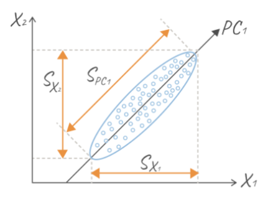
The blue dots forming, conditionally, an ellipse are data (each object has a pair of features). It seems like it's logical that along theline, the data change is most significant, isn't it? Why do we think so? But because along this straight line, obviously, the spread from the average (conditionally, from the center of the ellipse) is the largest. As a result, according to our idea, it is assumed that the greater the sample variance along the axis, the better the data changes. By itself, the idea of building a new coordinate system is not new, it echoes the idea and experience in analytical geometry: choose a convenient coordinate system, and the task will be solved many times easier.

Construction of the first main component

Definition 1. Centering – subtracting from each coordinate of each object the average of the values of this coordinate for all objects.

To begin with, it is always better to center the data, in fact, it has little effect, because we just shifted the center of the coordinate system, but this will simplify future calculations.

Let's consider some set of objectshaving two attributes. This means that each objectcan be identified with a vector having two coordinates $(x_{i1},x_{i2})$ that is, $x_i=(x_{i1},x_{i2}), i = {1, 2, ..., n}$ .

After changing the power of the basis to one, each objectwill correspond to a single coordinate $z_i: x_i=(x_{i1},x_{i2} )→z_i, i = {1, 2, ..., n}$ .

Then the new coordinates of all objects can be written as a column vector $Z_1=\begin{pmatrix} z_1 \\ ... \\ z_n\\ \end{pmatrix}$

Since we want to draw a new line so that the new coordinates differ from each other as much as possible, we will use sample variance as a measure of difference

$S^2(Z_1)=\frac{1}{n}\sum^n_{i=1}(z_i-Z_{mean})^2$ , where $Z_{mean}=\frac{1}{n}\sum^n_{i=1}z_i$ - sample average.

Definition 2. A straight line passing through the origin, the coordinates of the projections of the centered source objects on which have the largest sample variance, is called the first main component and is denoted

Definition 3. The guiding vector $\phi$ of the first main component, having length 1, is called the vector of weights of the first main component.

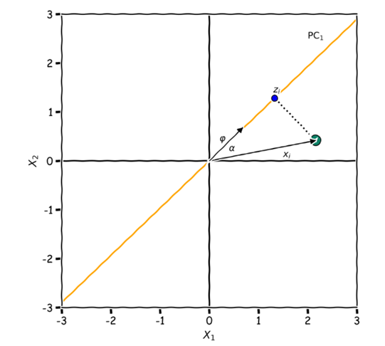
To find the new coordinate the line with the basis vector $\phi$ you can use the scalar product, which is defined as follows: $(x_i, \phi)=|x_i||\phi|cos(\alpha),$ where $\alpha$ is the angle between the vectorsand $\phi.$ Considering that $|\phi|=1, (x_i, \phi)=|x_i|cos(\alpha)=z_i.$ Or you can use $z_i=(x_i,\phi)=x_{i1}\phi_1+x_{i2}\phi_2.$ See the picture below.

So, our task is to find such weights $\phi_1, \phi_2,$ that is, to find a way to draw a straight line so that the coordinates of the projections of points on this line differ the most, that is, they have the greatest sample variance. We will discuss this a little later.

The second and subsequent main components

Let the initial feature space have dimension p >= 2 and it is necessary to construct not one, but k principal components. The first main component is constructed similarly to the example considered. The second and subsequent Main components are constructed so that they also pass through the origin, orthogonally to all previously constructed main components. The requirement of orthogonality of the main components ensures that there is no correlation between the new features of objects. At the same time, the next main component is constructed so that the sample variance of projections is maximal.

Finding the vector of weights of the first main component

Definition 4. Let n objectshave p features each, that is, $x_1=(x_{11}, x_{12}, ...,x_{1p}), x_2=(x_{21}, x_{22}, ...,x_{2p}),..., x_n=(x_{n1}, x_{n2}, ...,x_{np}).$ Then we will call the matrix of the initial data a matrix of size [n*p] of the form

$F=\begin{pmatrix} x_{11} & x_{12} & ... & x_{1p}\\ x_{21} & x_{22} & ... & x_{2p} \\ ... \\ x_{n1} & x_{n2} & ... & x_{np} \end{pmatrix}$

where in the i-th row of the matrix F are the corresponding features of the i–th object.

Next, we assume that the matrix F is obtained as a result of centering some initial matrix of objects F’.

Remark. Since we have p features, the guiding vector (the vector of weights) will also have p features: $\phi_1=(\phi_{11}, \phi_{21},...,\phi_{p1}).$ And since the length of the vector is equal to one, then

$|\phi| =\sqrt{\phi^2_{11}+\phi^2_{21}+...+\phi^2_{p1}} = 1 => \phi^2_{11}+ \phi^2_{21}+...+\phi^2_{p1} = 1.$

In matrix notation, we will write the coordinates of the vector $\phi_1$ in the form of a column

vector of the same name: $\phi_1=\begin{pmatrix} \phi_{11} \\ ... \\ \phi_{p1}\\ \end{pmatrix}.$

Definition 5. The vector of accounts of the first main component is a column vector of the form

$Z_1=\begin{pmatrix} z_{11} \\ ... \\ z_{n1}\\ \end{pmatrix},$ consisting of the coordinates of projections of centered source data on the

vector of weights of the first main component. In other words, the vector of accounts of the first main component is the new coordinates of objects relative to the first main component.

Theorem 1. Let

$F=\begin{pmatrix} x_{11} & x_{12} & ... & x_{1p}\\ x_{21} & x_{22} & ... & x_{2p} \\ ... \\ x_{n1} & x_{n2} & ... & x_{np} \end{pmatrix}$

be a matrix consisting of centered source data, and let $\phi_1$ be a vector of weights of the first principal component. Then the vector of accounts of the first principal component can be obtained from the relation $Z_1=F\phi_1.$ Provided that the sample variance of the resulting set is maximal.

Let me remind you that the sample variance of thesample can be found by the following

formula: $S^2(Z_1) =\frac{1}{n}\sum^n_{i=1}z^2_{i1}-(\frac{1}{n}\sum^n_{i=1}z_{i1})^2.$ Note that the right side of this difference can be

transformed as follows:

$\frac{1}{n}\sum^n_{i=1}z_{i1}=\frac{1}{n}\sum^n_{i=1}(\phi_{11}x_{i1} + \phi_{21}x_{i2}+...+\phi_{p1}x_{ip})=$

$=\phi_{11}\frac{1}{n}\sum^n_{i=1}x_{i1}+\phi_{21}\frac{1}{n}\sum^n_{i=1}x_{i2}+...+\phi_{p1}\frac{1}{n}\sum^n_{i=1}x_{ip}.$

But taking into account the fact that the features $x_{ij}$ are centered, which means their sample

averages are zero, that is $X_{j_{mean}} = \frac{1}{n}\sum^n_{i=1}x_{ij}=0, j = (1, 2, ..., p),$ we get that each term in

the last sum is zero. $\frac{1}{n}\sum^n_{i=1}z_{i1}=0=>(\frac{1}{n}\sum^n_{i=1}z_{i1})^2=0.$ Returning to the sample variance,

we get: $S^2(Z_1) =\frac{1}{n}\sum^n_{i=1}z^2_{i1} \to max_{\phi_1},$ in other words, we are looking for a vector of

weights such that the square of the lengthof the vector of accountsis maximal.

That is, $argmax_{\phi_1}(\frac{1}{n}\sum^n_{i=1}z^2_{i1})=argmax_{\phi_1}(\sum^n_{i=1}(\sum^p_{j=1}\phi_{j1}x_{ij})^2),$ provided that $|\phi_1|=1.$

Finding an arbitrary main component

Let the first main component $PC_1, p\geq2$ be constructed. The straight line passing through the origin orthogonally to the first main componentthe coordinates of the projections of the centered source objects on which have the greatest sample variance, is called the second main component and is denoted

And in general, let main components $PC_1, PC_2, ...,PC_{k-1}$ be constructed. The line passing through the origin orthogonally to each main component, the coordinates of the projections of the centered source objects on which have the largest sample variance, is called the k-th main component and is denoted

Similarly, as in the previous case, definitions of the guiding vector, the vector of accounts are introduced, and the formula for calculating the vector of accounts of the k-th main component remains the same.

A small conclusion on the calculation of the k-th main component

Summing up, the search for the k-th main component or, what is the same thing, the vector of weights $\phi_k,$ and, as a consequence, the vector of accounts is carried out according to the following algorithm:

1) It is stated that the vector has unit length, that is $\sum^p_{i=1}\phi^2_{ik}=\phi^2_{1k}+ \phi^2_{2k}+...+\phi^2_{pk} = 1.$

2) It is stated that the vector $\phi_k$ is orthogonal to each of the vectors of weights $\phi_1, \phi_2, ...,\phi_{k-1}.$

3) Then we solve the problem

$argmax_{\phi_k}(|Z_k|^2)=argmax_{\phi_1}(\frac{1}{n}\sum^n_{i=1}z^2_{ik})=argmax_{\phi_1}(\sum^n_{i=1}(\sum^p_{j=1}\phi_{jk}x_{ij})^2).$

4) After, using the formula $Z_k=F\phi_k,$ we calculate the vector of accounts of the k-th main component.

Example of finding the first main component

Suppose we have a table of elements that contain two attributes each:

Result (x(i))	attribute 1 (X’(1))	attribute 2 (X’(2))
1	9	19
2	6	22
3	11	27
4	12	25
5	7	22

Let's perform centering of features:

result (x(i))	attribute 1 (X’(1))	attribute 2 (X’(2))
1	0	-4
2	-3	-1
3	2	4
4	3	2
5	-2	-1

According to the written table, we will make a matrix:

$F_{5x2} = \begin{pmatrix} 0 & -4 \\ -3&-1\\2&4\\3&2\\-2&-1\end{pmatrix}$

Further, under the condition $\phi^2_{11}+\phi^2_{21}=1,$ and by the formula, we have

$F_{5x2} = \begin{pmatrix} 0 & -4 \\ -3&-1\\2&4\\3&2\\-2&-1\end{pmatrix} \begin{pmatrix} \phi_{11}\\ \phi_{21} \end{pmatrix}=\begin{pmatrix} -4\phi_{21}\\ -3\phi_{11}-\phi_{21} \\ 2\phi_{11}+4\phi_{21} \\ 3\phi_{11} + 2\phi_{21} \\ -2\phi_{11}-\phi_{21} \end{pmatrix}$

Now, we need to maximize the sample varianceThen, we get

$|Z_1|^2=(-4\phi_{21})^2+ (-3\phi_{11}-\phi_{21})^2 + (2\phi_{11}+4\phi_{21})^2 + (3\phi_{11} + 2\phi_{21})^2 + \\+(-2\phi_{11}-\phi_{21})^2$

Let's open the brackets and give similar terms. $|Z_1|^2=26\phi^2_{11}+38\phi_{11}\phi_{21} + 38\phi^2_{21}.$ We find

that when $\frac{\phi_{21}}{\phi_{11}}=\frac{6+\sqrt{397}}{19}$ the largest value of the function is reached.

Given a condition $\phi^2_{11}+\phi^2_{21}=1$ we find 2 pairs of solutions: $\phi_{11}\approx0.591, \phi_{21}\approx0.807$ or $\phi_{11}\approx-0.591, \phi_{21}\approx-0.807.$ We can choose any pair, since the difference is only in the direction. And now, we can calculate the new coordinates of the objects, relative to the first main component:

$F_{5x2} = \begin{pmatrix} 0 & -4 \\ -3&-1\\2&4\\3&2\\-2&-1\end{pmatrix} \begin{pmatrix} 0.591\\ 0.807 \end{pmatrix}=\begin{pmatrix} -3.226\\-2.580\\4.409\\3.387\\-1.989 \end{pmatrix}$

Since the direction of the first main component is given by the vector of weights $\phi_1,$ it is possible to construct an equation of a straight line: $X_2=\frac{\phi_{21}}{\phi_{11}}X_1=1.365X_1.$

Choosing the number of main components

Definition 9. A nonzero $\phi$ vector is called an eigenvector of the theta matrix if the relation is satisfied for a certain number of lambda: $\theta\phi=\lambda\phi.$ In this case, the lambda number is called the eigenvalue of the theta matrix.

Let's consider the sequence of actions for finding the main components. Let F be a centered matrix containing information about n objects with p features.

$F=\begin{pmatrix} x_{11} & x_{12} & ... & x_{1p}\\ x_{21} & x_{22} & ... & x_{2p} \\ ... \\ x_{n1} & x_{n2} & ... & x_{np} \end{pmatrix}$

1) Find a sample covariance matrix from the ratio $\theta = \frac{1}{n}(F^TF).$

2) Find the eigenvalues $\lambda_i$ of matrix $\theta, i=(1,2,...,p).$

3) Find the orthonormal eigenvectors $\phi_i$ of matrix $\theta,$ corresponding to the eigenvalues $\lambda_i$

4) Select the required number of main components. At the same time, as the vector of weights of the first main component, it is reasonable to take the eigenvector of the theta matrix corresponding to the largest eigenvalue of this matrix (so that the loss of initial information is the least). As a vector of weights, the second main component is an eigenvector corresponding to the second largest eigenvalue, and so on.

5) Find new coordinates of objects in the selected basis by performing multiplication $Z=F\Phi,$ given that the coordinates of the selected eigenvectors are columns of the matrix $\Phi$ , and in the first column $\Phi$ are the coordinates of the vector of weights corresponding to the largest eigenvalue of the theta matrix, in the second – the coordinates of the vector of weights corresponding to the second largest eigenvalue, and so on.

Remark. Note that the eigenvalues for $\lambda_i$ the selected main component are equal to the sample variances of the i-th accounts.

Definition 10. Let $\lambda_1\geq\lambda_2\geq...\geq\lambda_p\geq0$ be the eigenvalues of the covariance matrix, and the eigenvectors of the covariance matrix corresponding to the largest eigenvalues $\lambda_1,\lambda_2,...,\lambda_p$ are taken as the vectors of the weights of the first k main component. The value

$\delta_k=\frac{\sum^k_{i=1}\lambda_i}{\sum^p_{i=1}\lambda_i}$

is called the proportion of the explained variance.

Remark. It is easy to notice that $\delta_k$ it takes values from zero to one and shows which part of the variance is taken into account when using the first k main components relative to the entire variance. In other words, the closer it is to unity, the less information we lose about the original objects.

Example of finding the first main component

Suppose we have a table of elements that contain two attributes each:

Result (x(i))	attribute 1 (X’(1))	attribute 2 (X’(2))
1	9	19
2	6	22
3	11	27
4	12	25
5	7	22

Let's perform centering of features:

result (x(i))	attribute 1 (X’(1))	attribute 2 (X’(2))
1	0	-4
2	-3	-1
3	2	4
4	3	2
5	-2	-1

According to the written table , we will make a matrix:

$F_{5x2} = \begin{pmatrix} 0 & -4 \\ -3&-1\\2&4\\3&2\\-2&-1\end{pmatrix}$

Let's make a selective $\theta$ covariance matrix: $\theta = \frac{1}{n}(F^TF)=\frac{1}{5}\begin{pmatrix}26 & 19 \\ 19 & 38 \end{pmatrix}.$

Let's find the eigenvalues of this matrix. Recall that the eigenvalues are found from the condition that the determinant of the difference $\theta$ and $\lambda E$ is zero: $|\theta-\lambda E|=0,$ where E is the unit matrix. In our case:

$\begin{vmatrix} \frac{26}{5}-\lambda & \frac{19}{5} \\ \frac{19}{5} & \frac{38}{5} - \lambda \end{vmatrix} = 0.$

We get the following roots:

$\lambda_1=\frac{32+\sqrt{397}}{5}, \lambda_2=\frac{32-\sqrt{397}}{5}.$

Since we choose the maximum among all eigenvalues for the first principal component and by definition $\theta\phi=\lambda\phi,$ we get

$\begin{pmatrix}26 & 19 \\ 19 & 38 \end{pmatrix}\begin{pmatrix} \phi_{11}\\ \phi_{21} \end{pmatrix}=(32+\sqrt{397})\begin{pmatrix} \phi_{11}\\ \phi_{21} \end{pmatrix}$

And, accordingly, we will find the roots of this equation:

$\phi_{11}\approx\frac{0.733}{\sqrt{1^2+0.733^2}}\approx0.591, \phi_{21}\approx\frac{1}{\sqrt{1^2+0.733^2}}\approx0.807.$

Then, if $Z_1=F\phi_1,$ then we get the following expression for the accounts of the first main component:

$F_{5x2} = \begin{pmatrix} 0 & -4 \\ -3&-1\\2&4\\3&2\\-2&-1\end{pmatrix} \begin{pmatrix} 0.591\\ 0.807 \end{pmatrix}=\begin{pmatrix} -3.226\\-2.580\\4.409\\3.387\\-1.989 \end{pmatrix}$

Let’s find the proportion of the explained variance if we leave one main component:

$\delta_1=\frac{\lambda_1}{\lambda_1+\lambda_2}=\frac{32+\sqrt{397}}{(32 - \sqrt{397}) + (32+\sqrt{397})}\approx0.811$

We got about 0.8, a good result.

Conclusion

In this article, we examined the key idea of the principal component analysis, learnt how to find the vectors of the weights of the principal components, how to determine how much information we lost during transformation, and considered a couple of examples.

Tags:

Hubs: