Queries in PostgreSQL. Hashing

Queries in PostgreSQL. Hashing

So far we have covered query execution stages, statistics, sequential and index scan, and have moved on to joins.

The previous article focused on the nested loop join, and in this one I will explain the hash join. I will also briefly mention group-bys and distincs.

One-pass hash join

The hash join looks for matching pairs using a hash table, which has to be prepared in advance. Here's an example of a plan with a hash join:

EXPLAIN (costs off) SELECT *
FROM tickets t
  JOIN ticket_flights tf ON tf.ticket_no = t.ticket_no;

                QUERY PLAN
−−−−−−−−−−−−−−−−−−−−−−−−−−−−−−−−−−−−−−−−−−−
 Hash Join
   Hash Cond: (tf.ticket_no = t.ticket_no)
   −> Seq Scan on ticket_flights tf
   −> Hash
       −> Seq Scan on tickets t (5 rows)

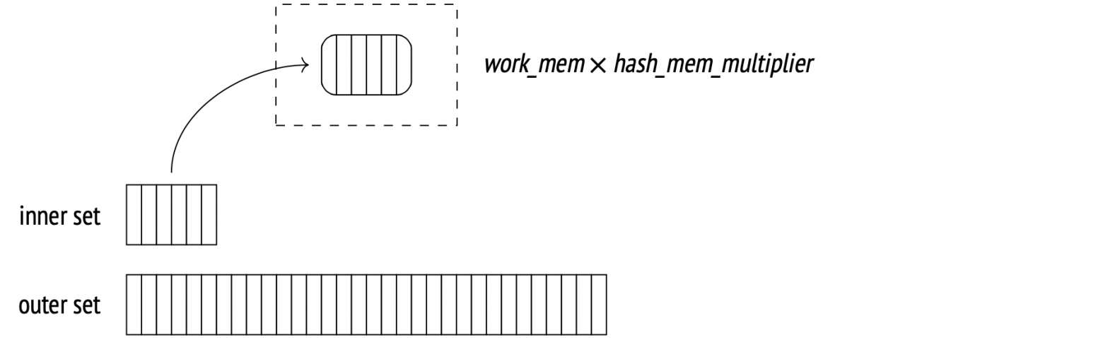
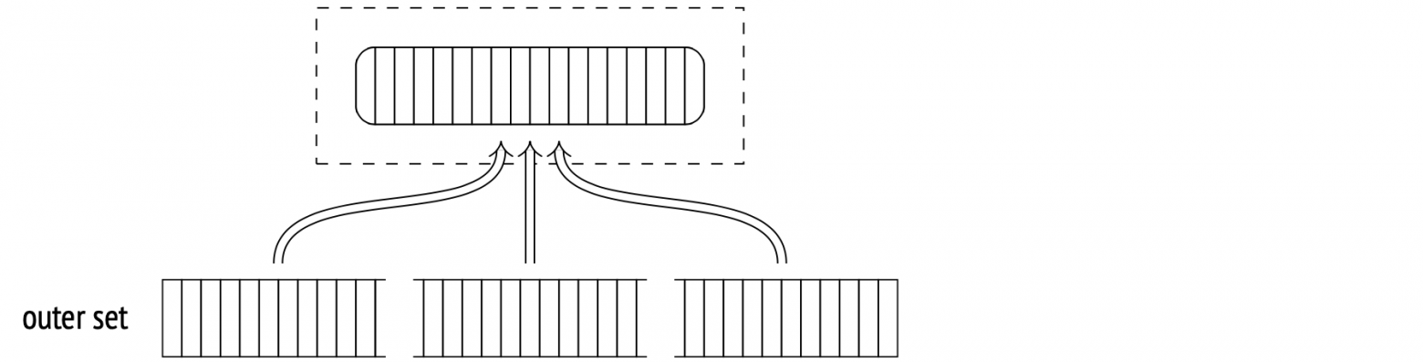
First, the Hash Join node calls the Hash node. The Hash node fetches all the inner set rows from its child node and arranges them into a hash table.

A hash table stores data as hash key and value pairs. This makes key-value search time constant and unaffected by hash table size. A hash function distributes hash keys randomly and evenly across a limited number of buckets. The total number of buckets is always two to the power N, and the bucket number for a given hash key is the last N bits of its hash function result.

So, during the first stage, the hash join begins by scanning all the inner set rows. The hash value of each row is computed by applying a hash function to the join attributes (Hash Cond), and all the fields from the row required for the query are stored in a hash table.

Ideally, the hash join wants to read all the data in one pass, but it needs enough memory for the entire hash table to fit at once. The amount of memory allocated for a hash table is work_mem × hash_mem_multiplier (the latter is 1.0 by default).

Let's use EXPLAIN ANALYZE and have a look at memory utilization:

SET work_mem = '256MB';
EXPLAIN (analyze, costs off, timing off, summary off)
SELECT *
FROM bookings b
  JOIN tickets t ON b.book_ref = t.book_ref;

                          QUERY PLAN
−−−−−−−−−−−−−−−−−−−−−−−−−−−−−−−−−−−−−−−−−−−−−−−−−−−−−−−−−−−−−−−
 Hash Join (actual rows=2949857 loops=1)
   Hash Cond: (t.book_ref = b.book_ref)
   −> Seq Scan on tickets t (actual rows=2949857 loops=1)
   −> Hash (actual rows=2111110 loops=1)
       Buckets: 4194304 Batches: 1 Memory Usage: 145986kB
       −> Seq Scan on bookings b (actual rows=2111110 loops=1)
(6 rows)

Unlike the nested loop join, which treats the inner and the outer sets differently, the hash join can easily swap the sets around. The smaller set is usually selected as the inner set because this way the hash table will be smaller.

In this case, the allocated memory was enough: the hash table took up about 143MB (Memory Usage), with 4 million (2²²) buckets. This allows the join to execute in one pass (Batches).

We can modify the query to select a single column. This will decrease the hash table size to 111MB:

EXPLAIN (analyze, costs off, timing off, summary off)
SELECT b.book_ref
FROM bookings b
  JOIN tickets t ON b.book_ref = t.book_ref;

                          QUERY PLAN
−−−−−−−−−−−−−−−−−−−−−−−−−−−−−−−−−−−−−−−−−−−−−−−−−−−−−−−−−−−−−−−
 Hash Join (actual rows=2949857 loops=1)
   Hash Cond: (t.book_ref = b.book_ref)
   −> Index Only Scan using tickets_book_ref_idx on tickets t
       (actual rows=2949857 loops=1)
       Heap Fetches: 0
   −> Hash (actual rows=2111110 loops=1)
       Buckets: 4194304 Batches: 1 Memory Usage: 113172kB
       −> Seq Scan on bookings b (actual rows=2111110 loops=1)
(8 rows)

RESET work_mem;

Yet another reason to be specific with your queries and try to avoid the SELECT * command.

The number of hash table buckets is selected in such a way as to have just one row per bucket, on average. A more compact distribution would increase the chance of hash collisions, and a more loose one would take up unnecessary amounts of memory. The minimum calculated number of buckets is increased to the closest power of two.

(With wide enough rows, the expected size of the hash table with an appropriate number of buckets can exceed the allocated memory. Whenever that happens, the algorithm splits the inner set into multiple batches and switches into the two-pass mode.)

No output can be returned until the first stage is complete.

During the second stage (after the hash table is built), the Hash Join node calls its second child node and fetches the outer set. For each fetched row, the hash table is probed for the matching rows, and a hash value is calculated for the join attributes (using the same hash function as before).

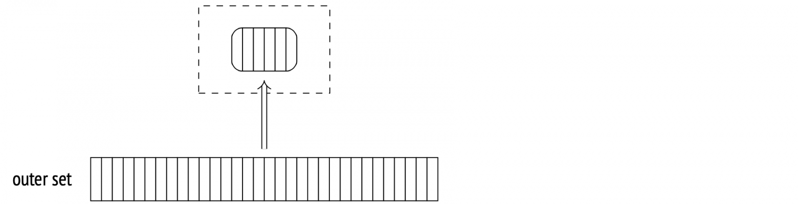
All matches and returned to the Hash Join node.

Now let's try a more branching plan with two hash joins. This query returns the names of all passengers and all their booked flights:

EXPLAIN (costs off)
SELECT t.passenger_name, f.flight_no
FROM tickets t
  JOIN ticket_flights tf ON tf.ticket_no = t.ticket_no
  JOIN flights f ON f.flight_id = tf.flight_id;

                  QUERY PLAN
−−−−−−−−−−−−−−−−−−−−−−−−−−−−−−−−−−−−−−−−−−−−−−−
 Hash Join
   Hash Cond: (tf.flight_id = f.flight_id)
   −> Hash Join
       Hash Cond: (tf.ticket_no = t.ticket_no)
       −> Seq Scan on ticket_flights tf
       −> Hash
           −> Seq Scan on tickets t
   −> Hash
       −> Seq Scan on flights f
(9 rows)

First, tickets are joined with ticket_flights, with a hash table built for tickets. Then, the resulting set is joined with flights, with a hash table built for flights.

Cost estimation. I've explained join cardinality in the previous article. The calculation is method-agnostic, so I won't repeat myself here. The cost estimation, however, is different.

The Hash node cost is considered equal to its child node cost. This is a dummy value used only in the plan output. All the real estimates are included within the Hash Join cost.

Consider this example:

EXPLAIN (analyze, timing off, summary off)
SELECT *
FROM flights f
  JOIN seats s ON s.aircraft_code = f.aircraft_code;

                             QUERY PLAN
−−−−−−−−−−−−−−−−−−−−−−−−−−−−−−−−−−−−−−−−−−−−−−−−−−−−−−−−−−−−−−−−−−−−−
 Hash Join  (cost=38.13..278507.28 rows=16518865 width=78)
   (actual rows=16518865 loops=1)
   Hash Cond: (f.aircraft_code = s.aircraft_code)
   −> Seq Scan on flights f  (cost=0.00..4772.67 rows=214867 widt...
       (actual rows=214867 loops=1)
   −> Hash  (cost=21.39..21.39 rows=1339 width=15)
       (actual rows=1339 loops=1)
       Buckets: 2048 Batches: 1 Memory Usage: 79kB
       −> Seq Scan on seats s  (cost=0.00..21.39 rows=1339 width=15)
           (actual rows=1339 loops=1)
(10 rows)

The startup cost is primarily the hash table building cost. It comprises:

• Full inner set fetch cost (we need that to build the table).
• Hash value calculation cost for each join field, for each inner set row (estimated at cpu_operator_cost per operation).
• Hash table insert cost for each inner set row (estimated at cpu_operator_cost per row).
• Startup outer set fetch cost (so that we have something to join with).

The total cost then adds the actual join costs:

• Hash value calculation cost for each join field, for each outer set row (estimated at cpu_operator_cost per operation).
• Join condition recheck cost (necessary to avoid hash collisions, estimated at cpu_operator_cost per operator).
• Output processing cost (cpu_operator_cost per row).

The interesting part here is determining exactly how many rechecks are necessary to complete the join. This number is estimated as the number of outer rows multiplied by a certain fraction of the number of inner rows (which reside in the hash table). The calculation is more complex than that and also depends on how uniform the data is. For our specific example, the fraction equals 0.150122, and I won't bore you with the exact details of the calculation.

With all that in mind, we can calculate the total cost estimate:

WITH cost(startup) AS (
  SELECT round((
    21.39 +
    current_setting('cpu_operator_cost')::real * 1339 +
    current_setting('cpu_tuple_cost')::real * 1339 +
    0.00
  )::numeric, 2)
)
SELECT startup,
  startup + round((
    4772.67 +
    current_setting('cpu_operator_cost')::real * 214867 +
    current_setting('cpu_operator_cost')::real * 214867 * 1339 *
      0.150112 +
    current_setting('cpu_tuple_cost')::real * 16518865
)::numeric, 2) AS total
FROM cost;

 startup |   total
−−−−−−−−−+−−−−−−−−−−−
   38.13 | 278507.26
(1 row)

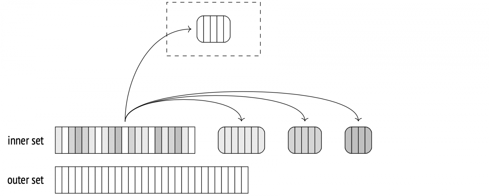
Two-pass hash join

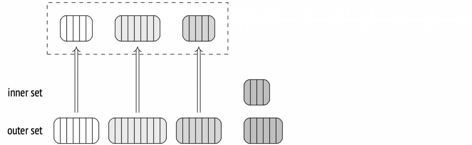
If the planner estimates that the hash table will not fit into the allocated memory, it splits the inner set into multiple batches and processes them separately. The total number of batches is always a power of two, and the ID of a batch is determined by the last bits of its hash value.

Any two matching rows belong in the same bucket, because rows from different buckets can't have the same hash value.

Each batch has the same number of hash values associated with it. If data is distributed uniformly, all buckets will be very close in size. The planner can control memory consumption by selecting a certain number of buckets in such a way that each single bucket will fit into available memory.

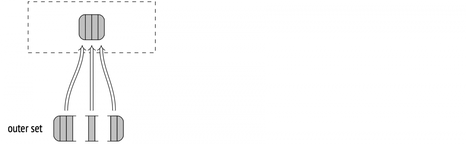
During the first stage, the algorithm scans the inner set and builds a hash table. If a scanned inner set row belongs to the first batch, the algorithm puts it into the hash table, so it remains in memory. Otherwise, if the row belongs to any other batch, it's stored in a temporary file (there's one for each bucket).

You can limit the size of temporary files created per session by using the temp_file_limit parameter (temporary tables are unaffected). Whenever a session exceeds the limit, it terminates.

During the second stage, the algorithm scans the outer set. If a scanned outer row belongs to the first batch, it is matched against the hash table, which stores the first batch of the inner set (there can be no matches in other batches anyway).

Otherwise, if the row belongs to another batch, it is stored in a temporary file (also separate for each batch). Therefore, with N total batches, the number of temporary files will be 2(N-1), less if any batches are empty.

When the outer set is scanned and the first batch is matched, the hash table is cleared.

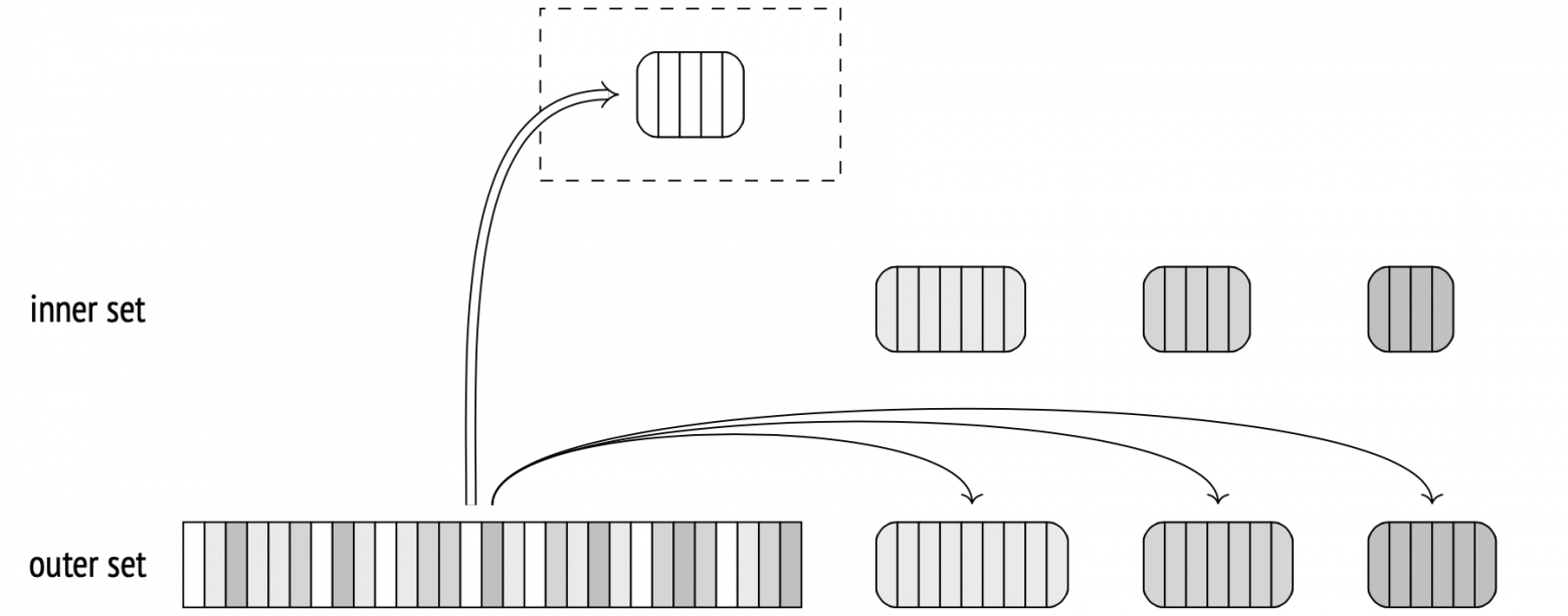
At this point, both sets are sorted into batches and stored in temporary files. From here on, the algorithm takes an inner set batch from its temporary file and builds its hash table, then takes the corresponding outer set batch from its temporary file and matches it against the table. When finished with the batch, the algorithm wipes both temporary files and the hash table, then repeats the procedure for the next batch, until completion.

Note that the number of batches in the EXPLAIN output for the two-pass join is larger than one. Additionally, the buffers option is used here to display disc usage statistics.

EXPLAIN (analyze, buffers, costs off, timing off, summary off)
SELECT *
FROM bookings b
  JOIN tickets t ON b.book_ref = t.book_ref;

                          QUERY PLAN
−−−−−−−−−−−−−−−−−−−−−−−−−−−−−−−−−−−−−−−−−−−−−−−−−−−−−−−−−−−−−−−
 Hash Join (actual rows=2949857 loops=1)
   Hash Cond: (t.book_ref = b.book_ref)
   Buffers: shared hit=7205 read=55657, temp read=55126
   written=55126
   −> Seq Scan on tickets t (actual rows=2949857 loops=1)
       Buffers: shared read=49415
       −> Hash (actual rows=2111110 loops=1)
           Buckets: 65536 Batches: 64 Memory Usage: 2277kB
           Buffers: shared hit=7205 read=6242, temp written=10858
           −> Seq Scan on bookings b (actual rows=2111110 loops=1)
               Buffers: shared hit=7205 read=6242
(11 rows)

This is the same example from before, but this time the default work_mem value is used. With just 4MB available, the hash table can't fit into the memory, so the algorithm decides to split it into 64 batches, with 64K buckets in total. When the hash table is built at the Hash node, the data is written into temporary files (temp written). During the join stage (the Hash Join node), the files are both read from and written into (temp read, temp written).

If you want more information on temporary files, you can set the log_temp_files parameter to zero. This will force the server to log a record of each file and its size upon deletion.

Dynamic plan adjustment

There are two possible issues that can mess up the plan. The first one is a non-uniform distribution.

If the values in the join key columns are distributed non-uniformly, different batches will have varying numbers of rows.

If the largest batch is any other but the first one, all the rows will have to be written on disk first and read from disk later. This is especially important for the outer set, as it usually is the larger one. Therefore, if we have the most common values statistics built for the outer set (in other words, if the outer set is a table and the join is done on one column, with no multivariate MCV lists), the rows with hash codes that match the MCV list are treated as belonging to the first batch. This is called skew optimization, and it helps reduce the input/output overhead during two-pass joining.

The second possible issue is outdated statistics.

Both issues may cause the size of some (or all) batches to be larger than expected, and the hash table may surpass the allocated memory as a result.

The algorithm can spot this during the table building stage and double the number of batches on the fly to avoid overflowing. Basically, it splits each batch in two. Half of the rows from each batch (assuming a uniform distribution) remains in memory, the other half is stored in a new temporary file on disk.

This could happen during one-pass joins as well. In fact, both one-pass and two-pass joins are governed by the same code. I'm only calling them differently to avoid confusion.

The number of batches can never decrease. If the planner has overestimated the batch sizes, it doesn't merge smaller batches together.

Splitting the batches may still prove inefficient when non-uniform distribution is at play. For example, the join key column may store the same value in every row. This will put all the rows in the same batch because the hash function will always return the same value. In this specific case there's nothing to do but watch the hash table grow, despite all the limiting parameters. In theory, this could be solved with a multi-pass join that checks a fraction of a batch at a time, but this has not been implemented yet.

To demonstrate the dynamic batch number increase, we will have to do something to trick the planner:

CREATE TABLE bookings_copy (LIKE bookings INCLUDING INDEXES)
WITH (autovacuum_enabled = off);
INSERT INTO bookings_copy SELECT * FROM bookings;

INSERT 0 2111110

DELETE FROM bookings_copy WHERE random() < 0.9;

DELETE 1899931

ANALYZE bookings_copy;
INSERT INTO bookings_copy SELECT * FROM bookings
ON CONFLICT DO NOTHING;

INSERT 0 1899931

SELECT reltuples FROM pg_class WHERE relname = 'bookings_copy';

 reltuples
−−−−−−−−−−−
    211179
(1 row)

We have just created a table bookings_copy. It is an identical copy of bookings, but the planner thinks it has ten times fewer rows than there actually are. A similar situation may occur in real life, when, for example, we build a hash table for a set of rows that itself is a result of another join with no accurate statistics for it.

We have managed to trick the planner into thinking that just 8 batches would be enough, while during the table building stage the number grows to 32:

EXPLAIN (analyze, costs off, timing off, summary off)
SELECT *
FROM bookings_copy b
  JOIN tickets t ON b.book_ref = t.book_ref;

                             QUERY PLAN
−−−−−−−−−−−−−−−−−−−−−−−−−−−−−−−−−−−−−−−−−−−−−−−−−−−−−−−−−−−−−−−−−−−−−
 Hash Join (actual rows=2949857 loops=1)
   Hash Cond: (t.book_ref = b.book_ref)
   −> Seq Scan on tickets t (actual rows=2949857 loops=1)
   −> Hash (actual rows=2111110 loops=1)
       Buckets: 65536 (originally 65536) Batches: 32 (originally 8)
       Memory Usage: 4040kB
       −> Seq Scan on bookings_copy b (actual rows=2111110 loops=1)
(7 rows)

Cost estimation. Here's the same example from the one-pass join section, but now I set an extremely low memory limit, forcing the planner to use two batches. This increases the cost:

SET work_mem = '64kB';
EXPLAIN (analyze, timing off, summary off)
SELECT *
FROM flights f
  JOIN seats s ON s.aircraft_code = f.aircraft_code;

                             QUERY PLAN
−−−−−−−−−−−−−−−−−−−−−−−−−−−−−−−−−−−−−−−−−−−−−−−−−−−−−−−−−−−−−−−−−−−−−
 Hash Join  (cost=45.13..283139.28 rows=16518865 width=78)
   (actual rows=16518865 loops=1)
   Hash Cond: (f.aircraft_code = s.aircraft_code)
   −> Seq Scan on flights f  (cost=0.00..4772.67 rows=214867 widt...
       (actual rows=214867 loops=1)
   −> Hash  (cost=21.39..21.39 rows=1339 width=15)
       (actual rows=1339 loops=1)
       Buckets: 2048 Batches: 2 Memory Usage: 55kB
       −> Seq Scan on seats s  (cost=0.00..21.39 rows=1339 width=15)
           (actual rows=1339 loops=1)
(10 rows)

RESET work_mem;

The join cost itself is increased by the temporary file writing and reading costs.

The startup cost will increase by the estimated cost of writing the number of pages sufficient to store the required fields from all the inner set rows. The first batch isn't written to disk when the hash table is built, but that is not taken into account by the estimate, so it doesn't depend on the number of batches.

The total cost is increased by the cost estimate for reading the stored inner set rows from disk and then writing and reading the outer set rows.

Both reading and writing are assumed to be sequential, and their costs for one row are estimated using the seq_page_cost parameter.

In this example, the number of pages for the inner set is estimated at 7, and for the outer set at 2309. By adding these costs to the one-pass estimate from before, we get the same estimate that the planner ends up with:

SELECT 38.13 + -- one-pass startup cost
  current_setting('seq_page_cost')::real * 7
  AS startup,
279232.27 + -- one-pass total cost
  current_setting('seq_page_cost')::real * 2 * (7 + 2309)
  AS total;

 startup |   total
−−−−−−−−−+−−−−−−−−−−−
   45.13 | 283864.27
(1 row)

This illustrates that when there's not enough memory available, the one-pass join algorithm becomes two-pass, and the efficiency suffers. To avoid the inefficiency, make sure that:

• The hash table only includes the truly necessary fields (responsibility of the programmer).
• The hash table is built for the smaller set (responsibility of the planner).

Hash join in parallel plans

Hash joins can work in parallel plans similarly to what I have described above. Each of the parallel processes will first build its own copy of the hash table from the inner set, and then use it to access the outer set in parallel. The benefit here is that each process only scans a fraction of the outer set.

Here's an example of a plan with a regular (one-pass, in this case) hash join:

SET work_mem = '128MB';
SET enable_parallel_hash = off;
EXPLAIN (analyze, costs off, timing off, summary off)
SELECT count(*)
FROM bookings b
  JOIN tickets t ON t.book_ref = b.book_ref;

                             QUERY PLAN
−−−−−−−−−−−−−−−−−−−−−−−−−−−−−−−−−−−−−−−−−−−−−−−−−−−−−−−−−−−−−−−−−−−−−
 Finalize Aggregate (actual rows=1 loops=1)
   −> Gather (actual rows=3 loops=1)
       Workers Planned: 2
       Workers Launched: 2
       −> Partial Aggregate (actual rows=1 loops=3)
           −> Hash Join (actual rows=983286 loops=3)
               Hash Cond: (t.book_ref = b.book_ref)
               −> Parallel Index Only Scan using tickets_book_ref...
                   Heap Fetches: 0
               −> Hash (actual rows=2111110 loops=3)
                   Buckets: 4194304 Batches: 1 Memory Usage:
                   113172kB
                   −> Seq Scan on bookings b (actual rows=2111110...
(13 rows)

RESET enable_parallel_hash;

Each process first makes a hash table for bookings. Then, the processes scan tickets in the Parallel Index Only Scan mode and match their sets of rows against the hash table.

The hash table size limit applies to each parallel process separately, so the total memory allocated will be (in this case) three times more than what the plan says under Memory Usage.

Parallel one-pass hash join

While the regular hash join may benefit from being run in parallel (especially with an inner set tiny enough to not be a concern for parallelization), the larger sets perform better with a dedicated parallel hash join algorithm, which has been introduced in PostgreSQL 11.

A significant advantage of the new algorithm is its ability to build the hash table in shared, dynamically allocated memory, which makes it accessible to all the participating parallel processes.

This allows all the processes to allocate their personal memory allowances towards building the shared table, instead of each building the same personal table. The larger memory pool can accommodate a larger table, increasing the chances that the whole table will fit and the join could be done in one pass.

During the first stage, under the Parallel Hash node, all the parallel processes scan the inner set in parallel and build a shared hash table.

Every process has to complete its part before the algorithm moves forward.

During the second stage (the Parallel Hash Join node), each process matches its part of the outer set with the shared hash table in parallel.

Here's an example of this at work:

SET work_mem = '64MB';
EXPLAIN (analyze, costs off, timing off, summary off)
SELECT count(*)
FROM bookings b
  JOIN tickets t ON t.book_ref = b.book_ref;

                            QUERY PLAN
−−−−−−−−−−−−−−−−−−−−−−−−−−−−−−−−−−−−−−−−−−−−−−−−−−−−−−−−−−−−−−−−−−−−−
 Finalize Aggregate (actual rows=1 loops=1)
   −> Gather (actual rows=3 loops=1)
       Workers Planned: 2
       Workers Launched: 2
       −> Partial Aggregate (actual rows=1 loops=3)
           −> Parallel Hash Join (actual rows=983286 loops=3)
              Hash Cond: (t.book_ref = b.book_ref)
              −> Parallel Index Only Scan using tickets_book_ref...
                  Heap Fetches: 0
              −> Parallel Hash (actual rows=703703 loops=3)
                  Buckets: 4194304 Batches: 1 Memory Usage: 115424kB
                  −> Parallel Seq Scan on bookings b (actual row...
(13 rows)

RESET work_mem;

This is the same query that we ran in the previous section, but I used the parameter enable_parallel_hash there to explicitly restrict this type of execution.

Despite having half the memory for the hash table compared to the previous example, this one executed in a single pass because of the shared memory feature (Memory Usage). The hash table here is a bit larger, but we don't need any others, so the total memory usage has decreased.

Parallel two-pass hash join

For a hash table large enough, even the shared memory of all the processes may not suffice to store it all at once. This fact may turn up during planning, or later, during the execution stage. When this occurs, another two-pass algorithm steps in, one very different from all the ones from before.

The major difference is that it uses a separate smaller hash table for each worker process instead of a single large hash table, and that each worker processes batches independently from the others. The smaller tables still reside in shared memory, accessible to other workers. If the algorithm discovers that the join operation isn't going to be a one-batch job during the planning stage, it builds the tables for each worker right away. If the insufficiency is discovered during the execution stage, the large table gets rebuilt into the smaller ones.

The first stage of the algorithm has the processes scan the inner set in parallel, split it into batches and write them into temporary files. Because each process scans only its portion of the inner set, none will build an entire hash table for any batch (including the first one). The entire set of rows of a batch is compiled into a dedicated file that all the processes write to as they sync up. This is why here, unlike with the non-parallel and parallel one-pass variations, every single batch gets stored on disk.

When all the processes are done with the hashing, the second stage begins. Here, the non-parallel algorithm would have started matching the outer set rows from the first batch with the hash table. The parallel one, however, doesn't have a full table yet, and has the batches processed independently. First, the algorithm scans the outer set in parallel, splits it into batches and stores the batches in separate temporary files on disk. At this stage, the scanned rows don't need a hash table built for them, so the number of batches will never increase.

When the processes are done scanning, the algorithm ends up with 2N temporary files storing inner and outer set batches.

Now, each process takes a batch and performs the actual join. It pulls the inner set from disk into the hash table, scans the outer set rows and matches them against the hash table rows. When done with the batch, the process selects another available batch, and so on.

If there are no unprocessed batches left, the process teams up with another process to help it finish up its batch. They can do that because all the hash tables reside in shared memory.

This approach outperforms the algorithm with a single large shared table, because the collaboration between processes is easier and the synchronization overhead is smaller.

Modifications

The hash join algorithm is not exclusive to inner joins; any other type of join, be it left, right, full, outer, semi- or anti-join, can utilize it just as well. The limitation, however, is that the join condition has to be an equality operator.

I have demonstrated some of the operations in the nested loop join example before. This is a right outer join example:

EXPLAIN (costs off) SELECT *
FROM bookings b
  LEFT OUTER JOIN tickets t ON t.book_ref = b.book_ref;

               QUERY PLAN
−−−−−−−−−−−−−−−−−−−−−−−−−−−−−−−−−−−−−−−−
 Hash Right Join
   Hash Cond: (t.book_ref = b.book_ref)
   −> Seq Scan on tickets t
   −> Hash
       −> Seq Scan on bookings b
(5 rows)

Note that the logical left join operation in the query transforms into a physical right join operation in the plan.

On the logical level, the bookings table would be the outer table (to the left of the equality operator), and the tickets table would be the inner one (to the right from the operator). If joined like that, the resulting table would include all the bookings without any tickets.

On the physical level, the planner determines which set is the inner one and which is the outer one not by their positions in the query, but by the relative join cost. This usually results in the set with the smaller hash table taking the inner spot, as is the case here with bookings. So, the join type switches from left to right in the plan.

It works the other way around, too. If you specify that you want a right outer join (to get all the tickets that have no associated bookings), the plan will use the left join:

EXPLAIN (costs off) SELECT *
FROM bookings b
  RIGHT OUTER JOIN tickets t ON t.book_ref = b.book_ref;

               QUERY PLAN
−−−−−−−−−−−−−−−−−−−−−−−−−−−−−−−−−−−−−−−−
 Hash Left Join
   Hash Cond: (t.book_ref = b.book_ref)
   −> Seq Scan on tickets t
   −> Hash
       −> Seq Scan on bookings b
(5 rows)

And a full join, to top it all off:

EXPLAIN (costs off) SELECT *
FROM bookings b
  FULL OUTER JOIN tickets t ON t.book_ref = b.book_ref;

               QUERY PLAN
−−−−−−−−−−−−−−−−−−−−−−−−−−−−−−−−−−−−−−−−
 Hash Full Join
   Hash Cond: (t.book_ref = b.book_ref)
   −> Seq Scan on tickets t
       −> Hash
           −> Seq Scan on bookings b
(5 rows)

The parallel hash join is not currently supported for the right and the left join (but it is being worked on). Note how in the next example the bookings table is used as the outer set. If the outer join was supported, it would have been selected as the inner set.

EXPLAIN (costs off) SELECT sum(b.total_amount)
FROM bookings b
  LEFT OUTER JOIN tickets t ON t.book_ref = b.book_ref;

                             QUERY PLAN
−−−−−−−−−−−−−−−−−−−−−−−−−−−−−−−−−−−−−−−−−−−−−−−−−−−−−−−−−−−−−−−−−−−−−
 Finalize Aggregate
   −> Gather
       Workers Planned: 2
       −> Partial Aggregate
           −> Parallel Hash Left Join
               Hash Cond: (b.book_ref = t.book_ref)
               −> Parallel Seq Scan on bookings b
               −> Parallel Hash
                   −> Parallel Index Only Scan using tickets_book...
(9 rows)

Grouping and distinct values

Grouping values for aggregation and removing duplicate values can be done by algorithms similar to the join algorithms. One of the approaches is to build a hash table for the required fields. Each value is placed in the table only if there is no such value in the table already. This results in a hash table containing only distinct values.

The planner node responsible for this approach is called HashAggregate.

Below are some examples. Number of seats by fare class (GROUP BY):

EXPLAIN (costs off) SELECT fare_conditions, count(*)
FROM seats
GROUP BY fare_conditions;

          QUERY PLAN
−−−−−−−−−−−−−−−−−−−−−−−−−−−−−−
 HashAggregate
   Group Key: fare_conditions
   −> Seq Scan on seats
(3 rows)

List of classes (DISTINCT):

EXPLAIN (costs off) SELECT DISTINCT fare_conditions
FROM seats;

          QUERY PLAN
−−−−−−−−−−−−−−−−−−−−−−−−−−−−−−
 HashAggregate
   Group Key: fare_conditions
   −> Seq Scan on seats
(3 rows)

Fare class plus another value (UNION):

EXPLAIN (costs off) SELECT fare_conditions
FROM seats
UNION
SELECT NULL;

             QUERY PLAN
−−−−−−−−−−−−−−−−−−−−−−−−−−−−−−−−−−−−
 HashAggregate
   Group Key: seats.fare_conditions
   −> Append
       −> Seq Scan on seats
       −> Result
(5 rows)

The Append node is where the sets of rows are combined, but it doesn't remove any duplicate values, which is something the UNION operation demands. This is done separately at the HashAggregate node.

Just like with a hash join, the amount of memory available for the hash table cannot exceed work_mem × hash_mem_multiplier.

If the hash table fits, the aggregation is done in one batch, as in this example:

EXPLAIN (analyze, costs off, timing off, summary off)
SELECT DISTINCT amount
FROM ticket_flights;

                          QUERY PLAN
−−−−−−−−−−−−−−−−−−−−−−−−−−−−−−−−−−−−−−−−−−−−−−−−−−−−−−−−−−−−−−−
 HashAggregate (actual rows=338 loops=1)
   Group Key: amount
   Batches: 1 Memory Usage: 61kB
   −> Seq Scan on ticket_flights (actual rows=8391852 loops=1)
(4 rows)

There aren't many distinct values, so the hash table takes up just 61KB (Memory Usage).

As soon as the table no longer fits into the memory, the excess values start getting spilled to disk, split into several partitions based on specific bits of their hash values. The number of partitions is always a power of two and is selected in such a way as to allow each partition's hash table to fit into the memory. The estimate is prone to statistical inaccuracies, so the resulting desired number of partitions gets multiplied by 1.5 for good measure, further decreasing the size of each partition and increasing the chance that it can be processed in a single batch.

As soon as the data set is scanned, the node returns the aggregation results for the values from the hash table.

Then, the hash table is wiped and the next partition is scanned from its temporary file and processed just like a regular set of rows. In some cases, a partition's hash table may overflow again. If this happens, the "extra" rows are once again split into partitions and stored on disk.

As you recall, the two-pass hash join algorithm moves all the most common values into the first batch to save some I/O time. There's no need to do that for aggregation because it only stores the overflowing rows on disk, not all of them. The most common values will probably show up in the set early enough and will secure a spot in the hash table anyway.

EXPLAIN (analyze, costs off, timing off, summary off)
SELECT DISTINCT flight_id
FROM ticket_flights;

                         QUERY PLAN
−−−−−−−−−−−−−−−−−−−−−−−−−−−−−−−−−−−−−−−−−−−−−−−−−−−−−−−−−−−−−−−
 HashAggregate (actual rows=150588 loops=1)
   Group Key: flight_id
   Batches: 5 Memory Usage: 4145kB Disk Usage: 98184kB
   −> Seq Scan on ticket_flights (actual rows=8391852 loops=1)
(4 rows)

In this example, the number of distinct values is high enough for the hash table to not fit into the memory limit. The data was processed in 5 batches: one for the initial set and four more for the four partitions stored on disk.

To be continued.