Have you ever looked for a flat? Would you like to add some machine learning and make a process more interesting?
Today we will consider applying Machine Learning for finding an optimal flat.
Introduction
First of all, I want to clarify this moment and explain what "an optimal flat" does mean. It is a flat with a set of different characteristics like "area", "district", "number of balconies" and so on. And for these features of the flat, we expect a specific price. Looks like a function which takes several parameters and returns a number. Or maybe a black box which provides some magic.
But… there is big "but", sometimes you can face a flat which is overpriced because of a set of reasons like a good geo-position. Also, there are more prestigious districts in the centre of a city and districts outside the town. Or… sometimes people want to sell their apartments because they move to another point of Earth. In other words, there are many factors which can affect the price. Does it sound familiar?
Little step aside
Before I continue, let me make a little lyrical digression.
I lived in the Yekaterinburg (the city between Europe and Asia, one of the cities which had held The Football World Championship in 2018) for 5 years.
I was in love with these concrete jungles. And I hated that city for winter and public transport. It is a growing city and every month there are thousands and thousands of flats to be sold.
Yes, it is an overcrowded, polluted city. At the same time - it is a good place for analysing a real estate market. I received a lot of advertisements for flats, from the Internet. And I will use that information to a further extent.
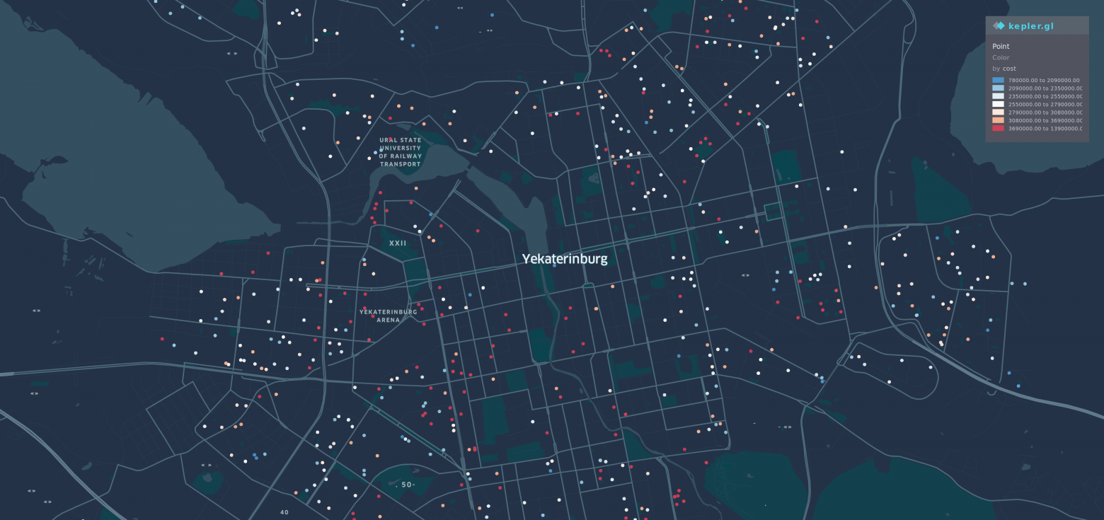
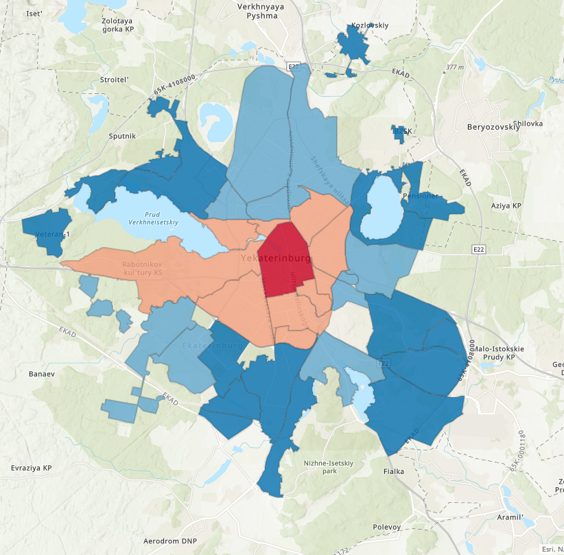
Also, I tried to visualize different offers on Yekaterinburg's map. Yes, it the catch-eye picture from habracut, it made on Kepler.gl
There are over 2 thousand 1-bedroom flat's which had been sold in July of 2019 in Yekaterinburg. They had a different price, from less than a million to almost 14 million roubles.
These points refer to their geo-position. Colour of points on the map represents the price, the lower is the price near to blue colour, the higher is the price near to red. You can consider it as an analogy with cold and warm colours, the warmer colour is the bigger is price.
Please, remember that moment, the redder is the colour, the higher is a value of something. The same idea works for blue but in the direction of the lowest price.
Now you are having a general overview of the picture and time to analyse is coming.
Goal
What did I want when l lived in Yekaterinburg? I looked for a good enough flat, or if we talk in terms of ML - I wanted to build a model which will give me a recommendation about buying.
On the one hand, if a flat is overpriced, the model should recommend waiting for price decreasing by showing the expected price for that flat.
On the other hand - if a price is good enough, according to the market state - perhaps I should consider that offer.
Of course, there is nothing ideal and I was ready to accept a mistake in calculations. Usually, for this kind of task use mean error of prediction and I was ready to 10% error. For example, if you have 2–3 million Russian roubles, you can ignore mistake in 200–300 thousand, you can afford it. As it seemed to me.
Preparing
As I mentioned before, there were a lot of apartments, let's look at them closely.
import pandas as pd
df = pd.read_csv('flats.csv')
df.shape
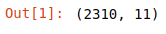
2310 flats for one month, we could extract something useful from that. What about a general data overview?
df.describe()
There is not something extraordinary - longitude, latitude, price of a flat(the label "cost"), and so on. Yes, for that moment I used "cost" instead of "price", I hope it will not lead to misunderstanding, please consider them as same.
Cleaning
Does every record have the same meaning? Some of them are represented flats like a cubicle, you can work there, but you would not like to live there. They are small cramped rooms, not a real flat. Let remove them.
df = df[df.total_area >= 20]
Prediction price of flat comes from the oldest issues in economics and related fields. There was nothing related to the term "ML" and people tried to guess price based on square meters/feet.
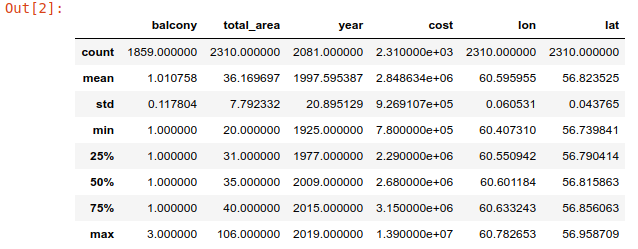
So, we look at these columns/labels and try to get the distribution of them.
numerical_fields = ['total_area','cost']
for col in numerical_fields:
    mask = ~np.isnan(df[col])
    sns.distplot(df[col][mask],  color="r",label=col)
    plot.show()
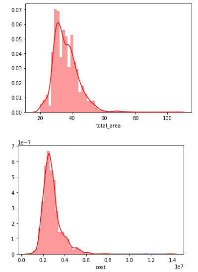
Well… there is nothing special, looks like a normal distribution. Perhaps we need to go deeper?
sns.pairplot(df[numerical_fields])
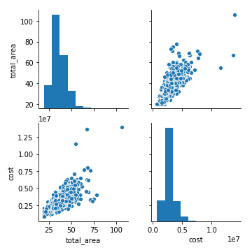
Oops… something wrong is there. Clean outliers in these fields and try to analyse our data again.
#Remove outliers
df = df[abs(df.total_area - df.total_area.mean()) <= (3 * df.total_area.std())]
df = df[abs(df.cost - df.cost.mean()) <= (3 * df.cost.std())]
#Redraw our data
sns.pairplot(df[numerical_fields])
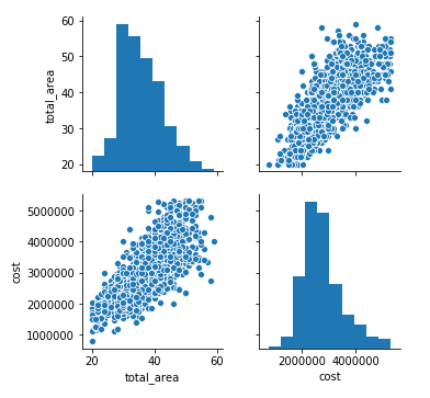
Outliers have gone, and now it looks better.
Transformation
The label "year", which is pointed at a year of construction should be transformed into something more informative. Let it be the age of building, in other words how a specific house is old.
df['age'] = 2019 -df['year']
Let have a look at the result.
df.head()
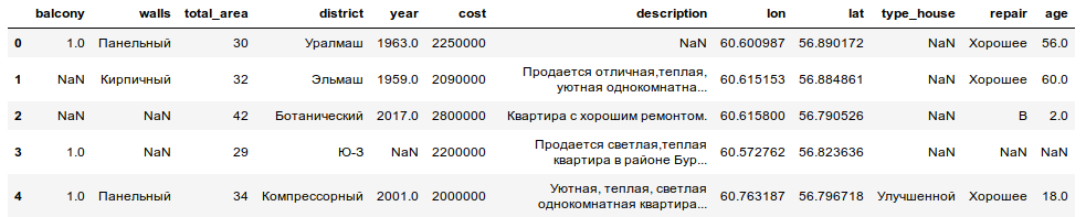
There are all kinds of data, categorical, Nan-values, text-description and some geo-information (longitude and latitude). Let us put aside the last ones because on that stage they useless. We will back to them later.
df.drop(columns=["lon","lat","description"],inplace=True)
Categorical data
Usually, for categorical data, people use different kinds of encoding or things like CatBoost which provide an opportunity to work with them as with numerical variables.
But, could we use something more logical and more intuitive? Now is time for making our data more understandable without losing the meaning of them.
Districts
Well, there are over twenty possible districts, could we add over 20 additional variables in our model? Of course, we could, but… should we? We are people and we could compare things, is not it?
First of all - not every district is equivalent to another. In the centre of city prices for one square meter is higher, further from downtown - it becomes to decrease. Does it sound logical? Could we use that?
Yes, definitely we could match any district with a specific coefficient and the further district is the cheaper flats are.
After matching the city and using another web service map(ArcGIS Online) changed and has a similar view
I used the same idea as for flat's visualization. The most "prestigious" and "expensive" district coloured in red and the least - blue. A colour temperature, do you remember about it?
Also, we ought to do some manipulation over our dataframe.
district_map =  {'alpha': 2,
                 'beta': 4,
                 ...
                 'delta':3,
                 ...
                 'epsilon': 1}
df.district = df.district.str.lower()
df.replace({"district": district_map}, inplace=True)
The same approach will be used for describing the internal quality of the flat. Sometimes it needs some repair, sometimes flat is quite well and ready for living. And in other cases, you should spend additional money on making it look better(to change taps, to paint walls). There also could be use coefficients.
repair = {'A': 1,
          'B': 0.6,
          'C': 0.7,
          'D': 0.8}
df.repair.fillna('D', inplace=True)
df.replace({"repair": repair}, inplace=True)
By the way, about walls. Of course, it also influences to price of flat. Modern material is better than older, brick is better than concrete. Walls from wood is quite a controversial moment, perhaps it is a good choice for the countryside, but not so good for urban life.
We use the same approach as before, plus make a suggestion about rows we do not know anything. Yes, sometimes people do not provide all the information about their flat. Furthermore, based on history we can try to guess about the material of walls. In a specific period of time (for example period Khrushchev's leading) - we know about typical material for building.
walls_map = {'brick': 1.0,
             ...
             'concrete': 0.8,
             'block': 0.8,
             ...
             'monolith': 0.9,
             'wood': 0.4}
mask = df[df['walls'].isna()][df.year >= 2010].index
df.loc[mask, 'walls'] = 'monolith'
mask = df[df['walls'].isna()][df.year >= 2000].index
df.loc[mask, 'walls'] = 'concrete'
mask = df[df['walls'].isna()][df.year >= 1990].index
df.loc[mask, 'walls'] = 'block'
mask = df[df['walls'].isna()].index
df.loc[mask, 'walls'] = 'block'
df.replace({"walls": walls_map}, inplace=True)
df.drop(columns=['year'],inplace=True)
Also, there is information about the balcony. In my humble opinion - the balcony is a really useful thing, so I could not help myself considering it.
Unfortunately, there are some null values. If the author of an advertisement had checked information about it, we would have more realistic information.
Well, if there is no information it will mean "there is not a balcony".
df.balcony.fillna(0,inplace=True)
After that, we drop columns with information about the year of building(we have a good alternative for its). Also, we remove column with information about the type of building because it has a lot of NaN-values and I have not found any opportunity to fill these gaps. And we drop all rows with NaN which we have.
df.drop(columns=['type_house'],inplace=True)
df = df.astype(np.float64)
df.dropna(inplace=True)
Checking
So… we used a not standard approach and replace categorical values to their numerical representation. And now we finished with a transformation of our data.
A part of the data has been dropped, but in general, it is a quite good dataset. Let look at the correlation between independent variables.
def show_correlation(df):
    sns.set(style="whitegrid")
    corr = df.corr() * 100
   # Select upper triangle of correlation matrix
    mask = np.zeros_like(corr, dtype=np.bool)
    mask[np.triu_indices_from(mask)] = True
   # Set up the matplotlib figure
    f, ax = plt.subplots(figsize=(15, 11))
   # Generate a custom diverging colormap
    cmap = sns.diverging_palette(220, 10)
   # Draw the heatmap with the mask and correct aspect ratio
    sns.heatmap(corr, mask=mask, cmap=cmap, center=0,
                linewidths=1, cbar_kws={"shrink": .7}, annot=True,
                fmt=".2f")
    plot.show()
    # df[columns] = scale(df[columns])
    return df
df1 = show_correlation(df.drop(columns=['cost']))

Erm… it became very interesting.
Positive correlation
Total area - balconies. Why not? If our flat is big there will be a balcony.
Negative correlation
Total area - age. The newer is flat, the bigger is an area for living. Sound logical, new are more spacious flat than older ones.
Age - balcony. The older is flat the fewer balconies it has. Seem like a correlation through another variable. Perhaps it is a triangle Age-Balcony-Area where one variable has an implicit influence on another. Put that on hold for a time.
Age - district. The older flat is the big probability that will be placed in the more prestigious districts. Could it be related to higher price near the centre?
Also, we could see the correlation with the dependent variable
plt.figure(figsize=(6,6))
corr = df.corr()*100.0
sns.heatmap(corr[['cost']],
            cmap= sns.diverging_palette(220, 10),
            center=0,
            linewidths=1, cbar_kws={"shrink": .7}, annot=True,
            fmt=".2f")

Here we go…
The very strong correlation between the area of flat and price. If you want to have a bigger place for living it will require more money.
There is a negative correlation between pairs "age/cost" and "district/cost". A flat in a newer house less affordable than the old one. And in the countryside flats are cheaper.
Anyhow, it seems clear and understandable, so I decided to go with it.
Model
For tasks related to prediction flat's price usually, use linear regression. According to significant correlation from a previous stage, we could try to use it as well. It is a workhorse which is suitable for many tasks.
Prepare our data for next actions
from sklearn.model_selection import train_test_split
y = df.cost
X = df.drop(columns=['cost'])
X_train, X_test, y_train, y_test = train_test_split(X, y, test_size=0.2, random_state=42)
Also, we create some simple functions for prediction and evaluation of the result. Let do our first try to predict price!
def predict(X, y_test, model):
    y = model.predict(X)
    score = round((r2_score(y_test, y) * 100), 2)
    print(f'Score on {model.__class__.__name__} is {score}')
    return score
def train_model(X, y, regressor):
    model = regressor.fit(X, y)
    return model
from sklearn.linear_model import LinearRegression
regressor = LinearRegression()
model = train_model(X_train, y_train, regressor)
predict(X_test, y_test, model)
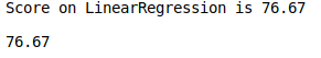
Well… 76.67% of accuracy. Is it a big number or not? According to my point of view, it is not bad. Moreover, it is a good starting point. Of course, it is not ideal, and there is a potential for improvement.
At the same time - we tried to predict only one part of the data. What about applying the same strategy for other data? Yes, time for cross-validation.
def do_cross_validation(X, y, model):
    from sklearn.model_selection import KFold, cross_val_score
    regressor_name = model.__class__.__name__
    fold = KFold(n_splits=10, shuffle=True, random_state=0)
    scores_on_this_split = cross_val_score(estimator=model, X=X, y=y, cv=fold, scoring='r2')
    scores_on_this_split = np.round(scores_on_this_split * 100, 2)
    mean_accuracy = scores_on_this_split.mean()
    print(f'Crossvaladaion accuracy on {model.__class__.__name__} is {mean_accuracy}')
    return mean_accuracy
do_cross_validation(X, y, model)

The result of the cross-validationNow we take another result. 73 is less than 76. But, it also a good candidate until a moment when we will have a better one. Also, it means that a linear regression works quite stable on our dataset.
And now is a time for the last step.
We will look at the best feature of linear regression - interpretability.
This family of models, in opposite to more complex ones, has a better ability to for understanding. There are just some numbers with coefficients and you can put your numbers in the equation, make some simple math and have a result.
Let try to interpret our model
def estimate_model(model):
    sns.set(style="white", context="talk")
    f, ax = plot.subplots(1, 1, figsize=(10, 10), sharex=True)
    sns.barplot(x=model.coef_, y=X.columns, palette="vlag", ax=ax)
    for i, v in enumerate(model.coef_.astype(int)):
        ax.text(v + 3, i + .25, str(v), color='black')
ax.set_title(f"Coefficients")
estimate_model(regressor)
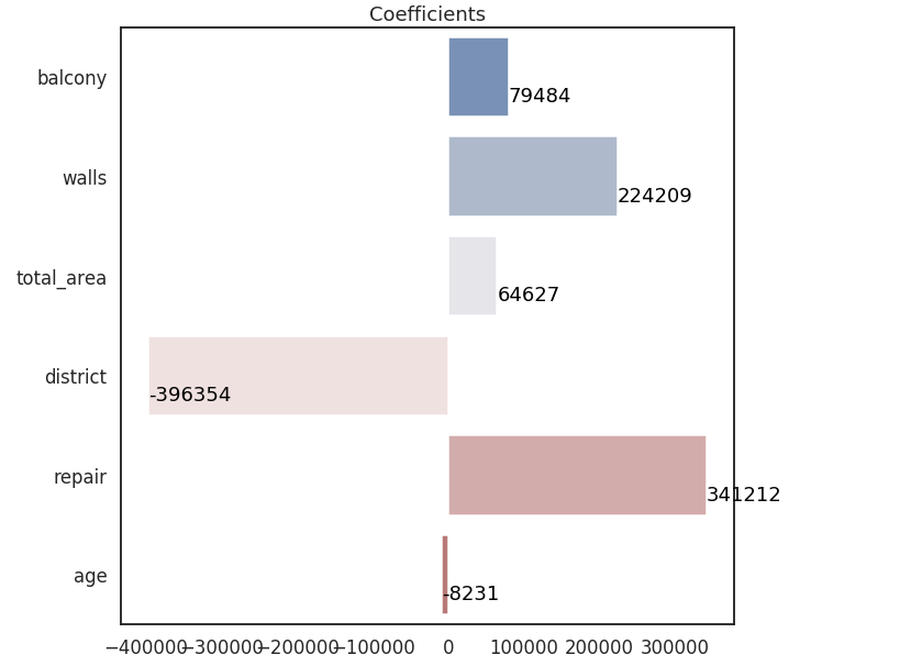
The picture looks quite logical. Balcony/Walls/Area/Repair give a positive contribution to a flat price.
The further flat is the bigger a negative contribution. Also applicable for age. The older flat is the lower price will be.
So, it was a fascinating journey.
We started from the ground, use the untypical approach for data transformation based on the human point of view(numbers instead dummy variables), checked variables and their relation to each other. After that, we build our simple model, used cross-validation for testing its. And as the cherry on the cake - look at the internals of model, what gives us confidence about our way.
But! It is not the finish our journey but only a break. We will try to change our model in the future and maybe (just maybe) it increases the accuracy of prediction.
Thanks for reading!
The second part is there
P.S. The source data and Ipython-notebook is located there
