Introduction
Hello, everyone! In this post, let's talk about how to (more) accurately measure the dynamic range of a camera sensor and what can be done with these measurements.
Of course, I am not an expert in computer vision, a programmer or a statistician, so please feel free to correct me in the comments if I make mistakes in this post. Here my interest was primarily focused on everyday and practical tasks, such as photography, but I believe the results may also be useful to computer vision professionals.
Update: mistakes were found here after publishing this post on the DPReview forum. I think it is important to note that here, and here is the link to the thread itself
Existing Problem
The dynamic range of modern image sensors is limited; we cannot capture detail in very bright highlights and very dark shadows simultaneously without degrading the image quality due to noise. In general, the noise, in my opinion, is the most limiting factor for image quality today. The darker the scene, the more noise there is in the shadows, which when the image becomes darker increases in amplitude more and more, progressively “eating away” detail, especially that of low‑contrast objects.
Why Measure Dynamic Range
In general, accurate dynamic range measurements can be used by both photographers (not only enthusiasts but also professionals) and computer vision specialists to evaluate some equipment.
Firstly, measurements help to answer the question of which camera or sensor to choose for the future tasks or whether an upgrade is worth it — to what extent the advantage will be noticeable. Secondly, through measurements, one can analyze an existing camera or sensor to find an optimal exposure and post‑processing strategy and also use the data for further research.
How Sensor Dynamic Range is Currently Measured
In this chapter, I am using the method and data from Bill Claff's website, Photons to Photos.
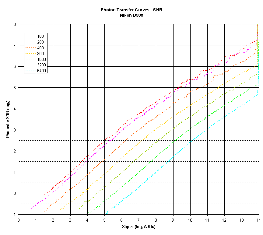
The current method of measuring dynamic range begins with the plotting of a graph of the signal-to-noise ratio for a specific ISO at different exposure values, as illustrated below:
In general, there are engineering and so-called photographic dynamic ranges. Here is what Mr. Claff writes regarding the first:
The low endpoint for Engineering Dynamic Range is determined by where the SNR curve crosses the value of 1.
Here is an extreme close-up of that area of the Photon Transfer Curve:

The ISO 100 line crosses 0 (the log2(1)) at 1.63 EV.
So Engineering Dynamic Range is 14.00 EV — 1.63 EV = 12.37 EV.
Or, if we use the White Level (from White Level), (14.00 EV — 0.11 EV) — 1.63 EV = 12.26 EV.
For comparison, here is the definition of the so-called photographic dynamic range:
My definition of Photographic Dynamic Range is a low endpoint with an SNR of 20 when adjusted for the appropriate Circle Of Confusion (COC) for the sensor.
For the D300 the SNR values on this curve is for a 5.5 micron square photosite.
To correct for a COC of.022mm we are looking for a log2 SNR value of 2.49.
Here is an close‑up of the area of the curve:
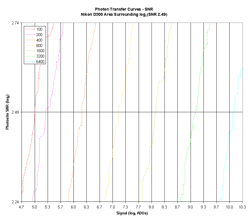
Note that the ISO 100 crosses 2.49 at 5.00 EV.
So Photographic Dynamic Range at ISO 100 is 14.00 EV — 5.00 EV = 9.00 EV.
Or, if we use the White Level (from White Level), (14.00 EV — 0.11 EV) — 5.00 EV = 8.89 EV.
The graphs obtained after such measurements can be found here — Photographic Dynamic Range versus ISO Setting.
For example, here is what the data looks like for the Pentax K-1:
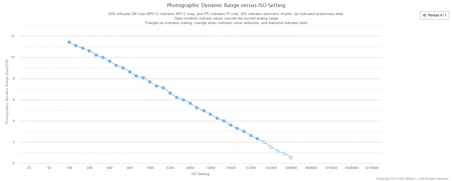
However, choosing an exposure strategy based solely on this graph is not the best idea because some cameras are so‑called ISO‑less. This means that increasing the ISO in the camera before capturing the image will not improve the noisy shadow detail but will only destroy highlight one.
Therefore, another graph is needed as well — such as this one — that shows shadow improvement versus ISO setting:
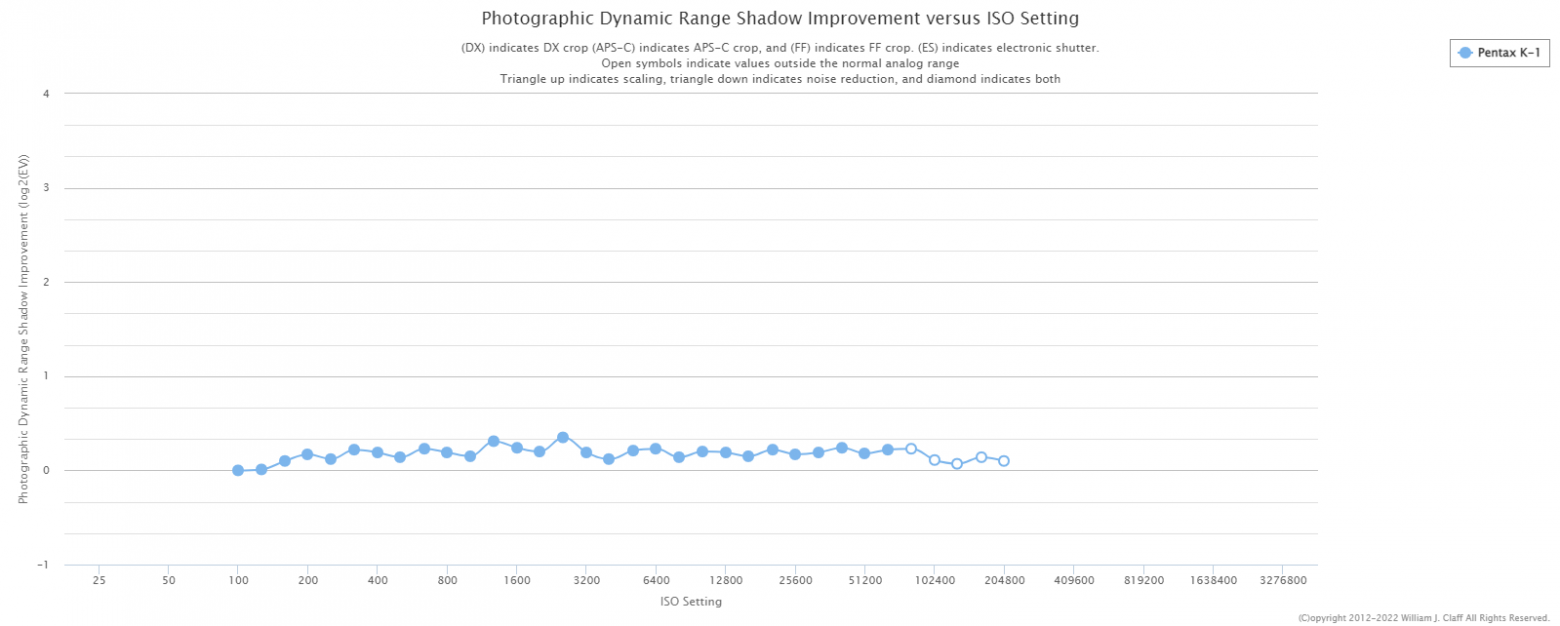
Indeed, the chosen camera turned out to be ISO‑less, meaning that increasing ISO beyond 100 will not improve the shadow detail.
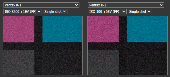
For clarity, here are two frames from the same camera by DPReview — one at ISO 3200 with exposure increased by one stop, and another at ISO 100 with exposure increased by 6 stops:
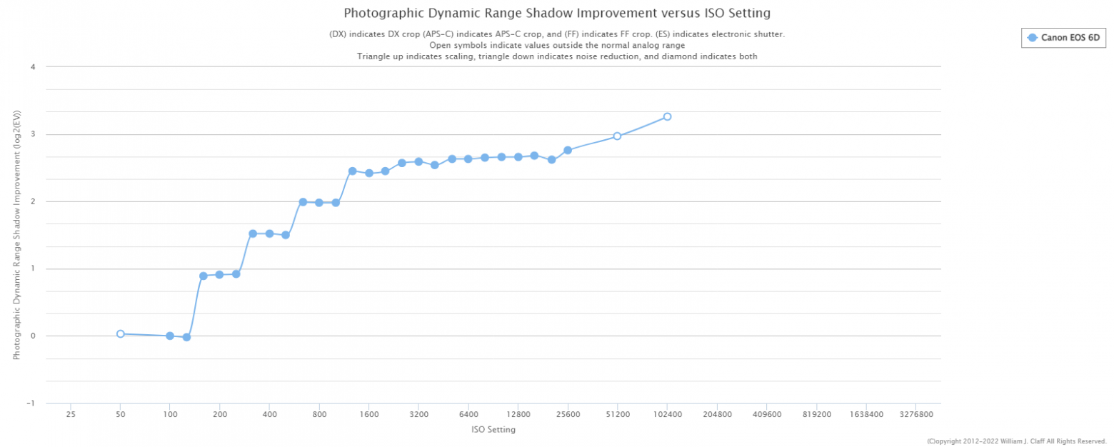
But this doesn't apply to all cameras. For example, here is the Canon 6D, increasing ISO indeed improves the shadows:
One cannot say that the camera is necessarily better or worse solely because of this characteristic, but it does influence the choice of an optimal exposure strategy during shooting.
Shortcoming of Such Measurement Method
The problem with such a classical approach arises when a camera uses noise reduction. Yes, these are still RAW files, it's just that noise reduction can be applied even before demosaicing. As seen in the graph below, the dynamic range sharply increases at ISO 640:

This does not necessarily mean that the image quality has actually improved. On the contrary, noise reduction could have destroyed some fine detail.
On the Shadow Improvement chart, the advantage is even more apparent — reaching almost 2 stops:
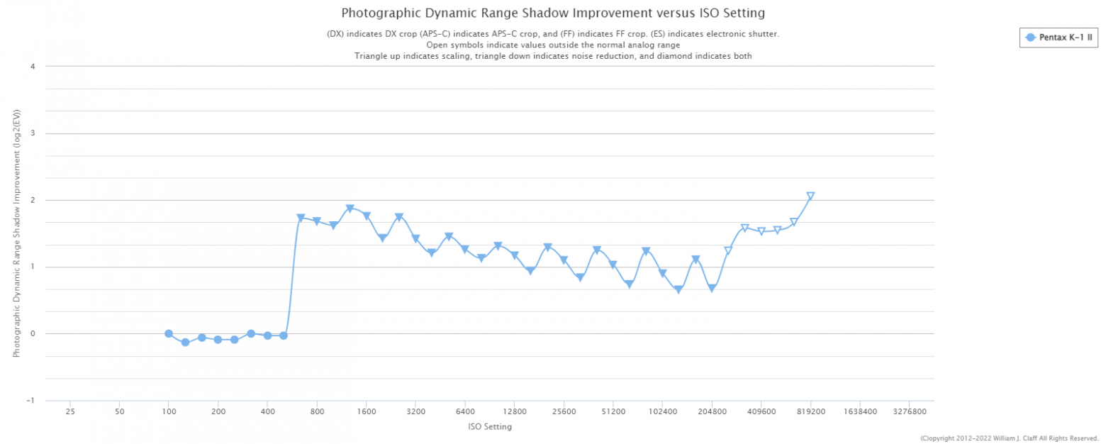
In reality, as you understand, things won't be as great. This is the problem with the classical measurement approach — DSP algorithms, such as noise reduction and detail recovery, can only be detected (which is what the triangles pointing down on the graph represent), but their actual impact on image quality cannot be accurately assessed.
A more advanced method of dynamic range measurement
You are likely familiar with the libraw library, and perhaps even use it. The developer of this library, Alexey Tutubalin (Алексей Тутубалин), proposed his way of measuring dynamic range back in 2017. He pondered the question of how much real resolution remains in an image due to the influence of noise. For this, Alexey used a low‑contrast rotated target to test the resolution. The rotation was introduced to challenge the internal DSP algorithms in the camera, in case such algorithms were present. It looked like this:


After a series of shots and a semi-automatic analysis of results, this interesting graph was obtained:
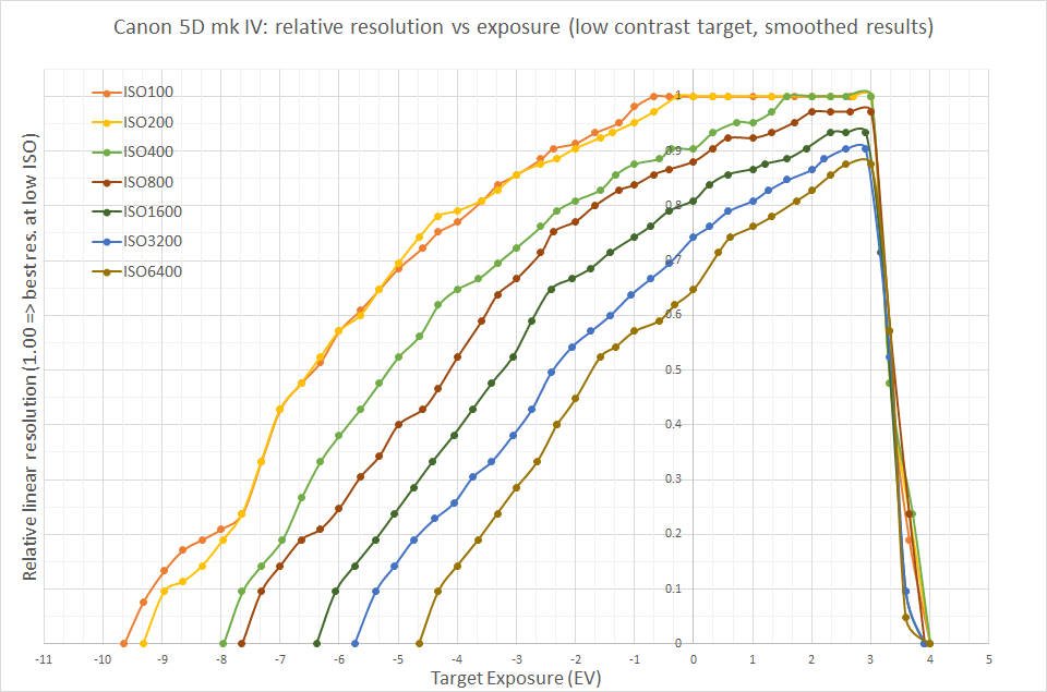
In my opinion, the data turned out to be incredibly useful and illustrative, but I wanted to replicate the results using fully automated measurements and metrics, ensuring that the developed method is accessible to everyone in home conditions.
Proposed Solution
I believe that testing resolution using special targets might lead to potential cheating attempts by the camera. The target should have resolution, i.e., detail, higher than that of a sensor. Therefore, we need a target with a large number of small details that cannot be tampered with — essentially just noise. However, we cannot use ordinary noise, as it would decrease as the camera moves away from the target. So, we need a special, scale‑invariant pink noise.
Imatest sells such targets for $330:
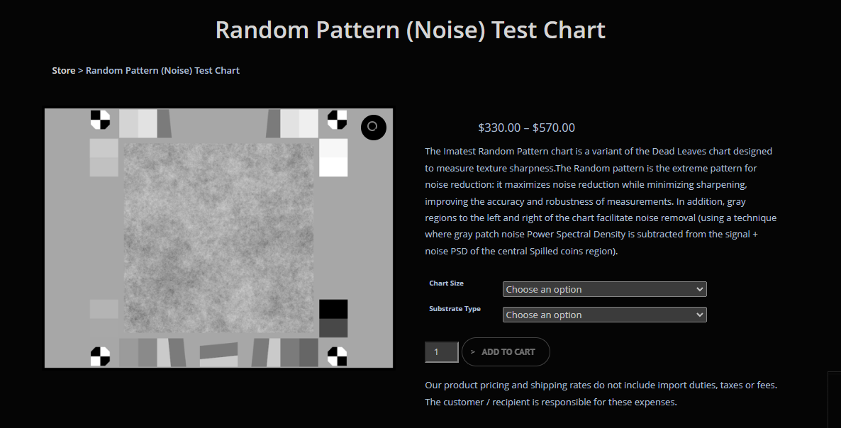
I just printed such a square on a regular printer on an A4 sheet.
Unfortunately, I don't have a standalone camera, so the testing was done on a regular phone with a SONY IMX686 sensor. I used the FreeDCam app, controlled it from a PC using scrcpy to avoid moving the phone between frames (in the case of a real camera, it would need to be placed on a tripod and remotely controlled from the PC). After that, I took series of shots of the resulting target at different ISOs with different exposures, from 1 to 12 stops below sensor saturation (careful readers will notice that, in fact, the lines on the graph are cut off before 12 stops at ISO 3200 and 6400 — FreeDCam simply does not have such short exposure time settings). The captured frames were converted into linear 16-bit TIFF without demosaicing but with white balance applied through channel amplification. Then they were analyzed relative to the reference frame — 10 averaged frames of the target taken at one stop below sensor saturation — equivalent to a frame at ISO 5 with ideal exposure.
The resulting graph shows the signal‑to‑noise ratio:
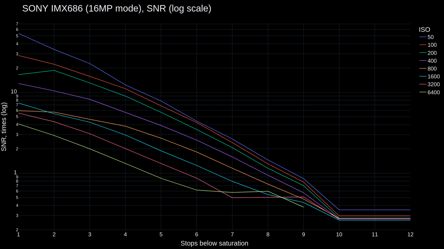
Unlike Mr. Claff's graph, this graph, if not entirely, at least partially, is resistant to DSP — please pay attention to the lower values at ISO 3200 and 6400, which are likely signs of noise reduction. Although the graph is not entirely free from its influence, there is no improvement relative to the upper values. Therefore, the obtained data has higher quality than the one that would be obtained by the standard method. In fact, I tested my phone without actual pink noise, so using real pink noise (which can be generated, for example, using functions from here) will likely only improve the result.
Instead of plotting graphs the classical way, I decided to go further and plot a graph similar to Alexey Tutubalin's, again using data obtained fully automatically and, as I hope, with greater accuracy. For this, I wrote and used this numpy function:
def find_real_resolution(image_resolution, ground_truth, noisy_image):
     stock_contrast = np.max(ground_truth) / np.min(ground_truth)
     noise = np.mean(np.abs(noisy_image - ground_truth))
     real_contrast = (np.max(ground_truth) - noise) / (np.min(ground_truth) + noise)
     contrast_change_coefficient = stock_contrast / real_contrast
     real_resolution = image_resolution / contrast_change_coefficient
     return real_resolution
More about it:
image_resolution - the resolution of the entire frame (as in this case only a cropped part of 100x100 pixels was tested), ground_truth - the reference image, noisy_image - the tested image from the series. As you understand, all frames in the series just need to be passed through this function. But what does it do?
Let's take another look at the resolution test target:

In the worst case, noise will decrease the value of the white background and increase the value of the black lines, leading to a reduction in contrast, and consequently a drop in the resolution for the given target. Therefore, I first find the “average noise” of each frame (line 2 inside the function), then subtract it from the white point of the reference image and add it to the black point of the same image (line 3). Then, I compare (line 4) the original (line 1) and the new (line 3) contrast, after which I simply divide (line 5) the entire frame's resolution by this coefficient to obtain the actual resolution.
The resulting graph looks like this:
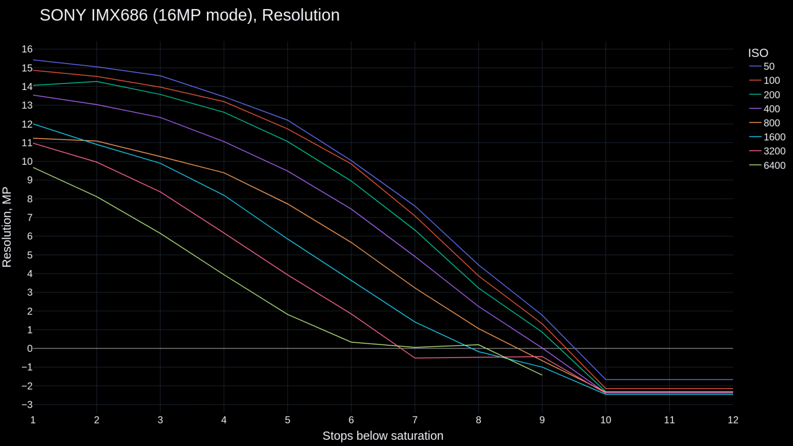
Values below 0 are shown for illustrative purposes only.
As mentioned earlier, such a graph can be used to compare two sensors to understand, for example, which one to choose for specific lighting conditions. Alternatively, one can investigate the graph of a single sensor to determine the optimal exposure strategy and to develop the best post‑processing algorithms, such as noise reduction.
Further Research
For a further work I would like to note the following opportunities:
Splitting Bayer filter into channels before the analysis. If the camera's autofocus pixels are only blue ones, it would be interesting to compare them with those without autofocus (e.g., one of the green channels).
Using this method for processed, non‑RAW images. This would be useful not only for visually evaluating the performance of noise reduction algorithms in post‑processing but also for understanding how much real detail they preserve. It could aid in the development of new algorithms related to detail recovery and noise reduction, possibly even neural network‑based.
Modification of the method for video use. It could involve displaying new pink noise images frame by frame on a high‑refresh‑rate monitor. However, the program analyzing such video should know when each frame was displayed. This could be achieved by providing auxiliary information (e.g., frame number, possibly encoded in a QR code) alongside the main target. Such a system would be resistant to temporal noise reduction methods commonly used in video.
Employing more accurate calculations, possibly relying on statistical analysis, to determine real resolution.
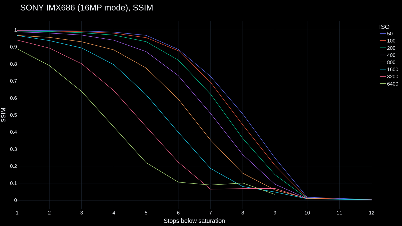
Using different image quality evaluation metrics to present results. For example, here is SSIM:
That's all for now, thanks for reading!