
With the advent of mobile phones with high-quality cameras, we started making more and more pictures and videos of bright and memorable moments in our lives. Many of us have photo archives that extend back over decades and comprise thousands of pictures which makes them increasingly difficult to navigate through. Just remember how long it took to find a picture of interest just a few years ago.
One of Mail.ru Cloud’s objectives is to provide the handiest means for accessing and searching your own photo and video archives. For this purpose, we at Mail.ru Computer Vision Team have created and implemented systems for smart image processing: search by object, by scene, by face, etc. Another spectacular technology is landmark recognition. Today, I am going to tell you how we made this a reality using Deep Learning.
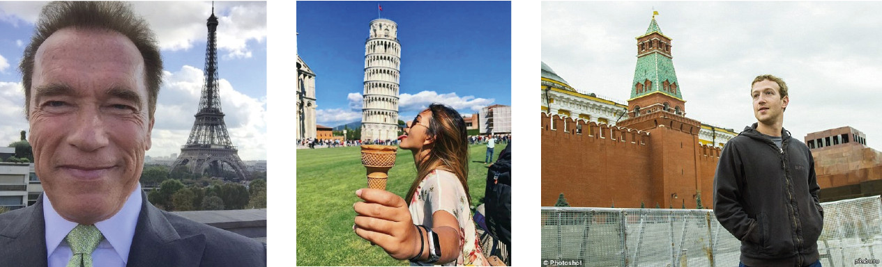
Imagine the situation: you return from your vacation with a load of photos. Talking to your friends, you are asked to show a picture of a place worth seeing, like palace, castle, pyramid, temple, lake, waterfall, mountain, and so on. You rush to scroll your gallery folder trying to find one that is really good. Most likely, it is lost amongst hundreds of images, and you say you will show it later.
We solve this problem by grouping user photos in albums. This will let you find pictures you need just in few clicks. Now we have albums compiled by face, by object and by scene, and also by landmark.
Photos with landmarks are essential because they often capture highlights of our lives (journeys, for example). These can be pictures with some architecture or wilderness in the background. This is why we seek to locate such images and make them readily available to users.
Peculiarities of landmark recognition
There is a nuance here: one does not merely teach a model and cause it to recognize landmarks right away — there are a number of challenges.
First, we cannot tell clearly what a “landmark” really is. We cannot tell why a building is a landmark, whereas another one beside it is not. It is not a formalized concept, which makes it more complicated to state the recognition task.
Second, landmarks are incredibly diverse. These can be buildings of historical or cultural value, like a temple, palace or castle. Alternatively, these may be all kinds of monuments. Or natural features: lakes, canyons, waterfalls and so on. Also, there is a single model that should be able to find all those landmarks.
Third, images with landmarks are extremely few. According to our estimations, they account for only 1 to 3 percents of user photos. That is why we can’t afford to make mistakes in recognition because if we show somebody a photograph without a landmark, it will be quite obvious and will cause an adverse reaction. Or, conversely, imagine that you show a picture with a place of interest in New York to a person who has never been to the United States. Thus, the recognition model should have low FPR (false positive rate).
Fourth, around 50 % of users or even more usually disable geo data saving. We need to take this into account and use only the image itself to identify the location. Today, most of the services able to handle landmarks in some way use geodata from image properties. However, our initial requirements were more stringent.
Now let me show you some examples.
Here are three look-alike objects, three Gothic cathedrals in France. On the left is Amiens cathedral, the one in the middle is Reims cathedral, and Notre-Dame de Paris is on the right.
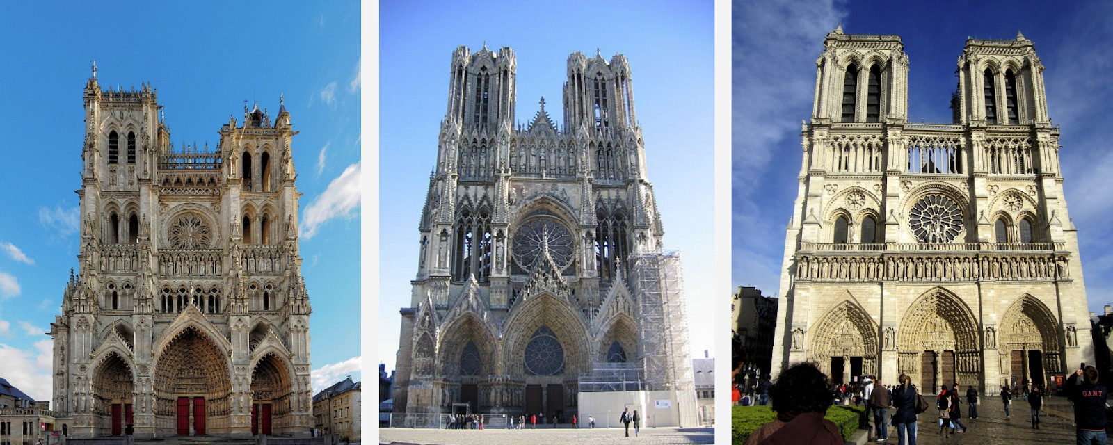
Even a human needs some time to look closely and see that these are different cathedrals, but the engine should be able to do the same, and even faster than a human does.
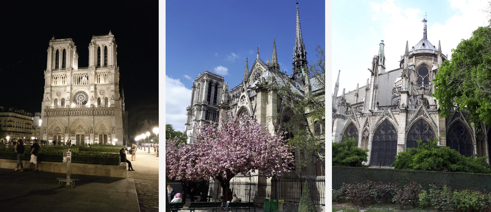
Here is another challenge: all the three photos here feature Notre-Dame de Paris shot from different angles. The photos are quite different, but they still need to be recognized and retrieved.
Natural features are entirely different from architecture. On the left is Caesarea in Israel, on the right is Englischer Garten in Munich.
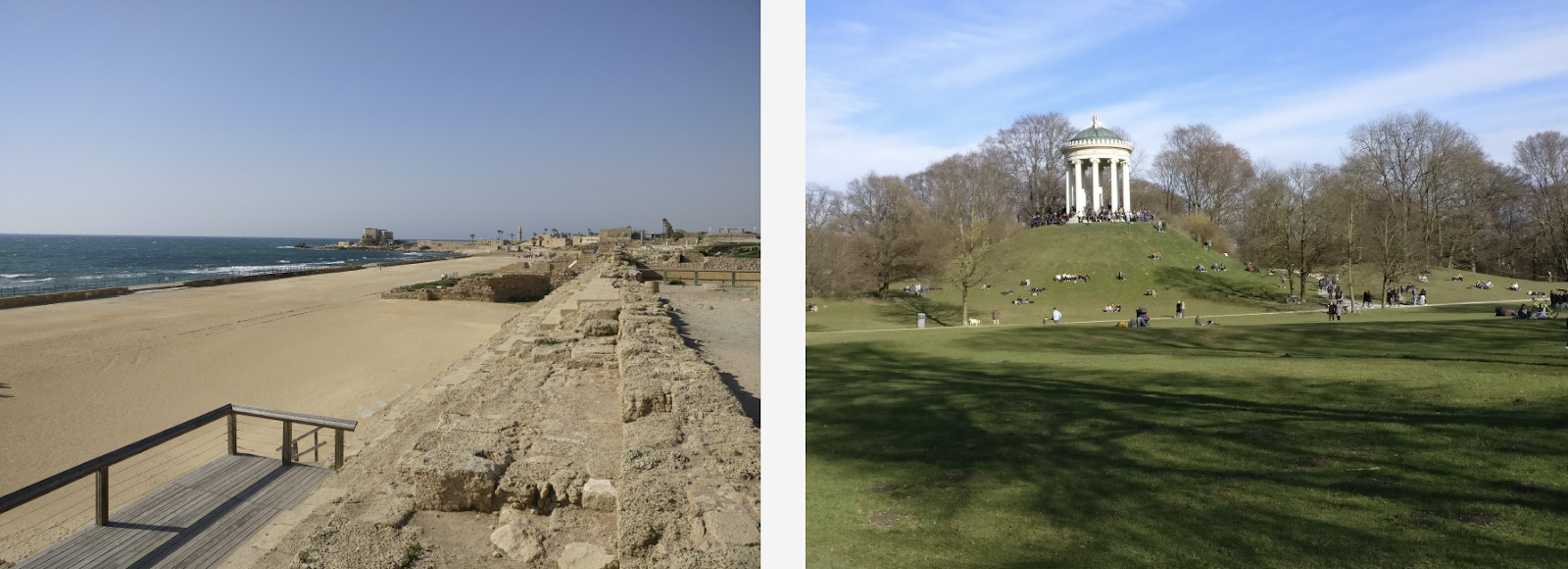
These photos give the model very few clues to guess.
Our method
Our method is based completely on deep convolutional neural networks. The training strategy we chose was so-called curriculum learning which means learning in several steps. To achieve greater efficiency both with and without geo data available, we made a specific inference. Let me tell you about each step in more detail.
Data set
Data is the fuel of machine learning. First of all, we had to get together data set to teach the model.
We divided the world into 4 regions, each being used at a specific step in the learning process. Then, we selected countries in each region, picked a list of cities for each country, and collected a bank of photos. Below are some examples.
First, we attempted to make our model learn from the database obtained. The results were poor. Our analysis showed that the data was dirty. There was too much noise interfering with recognition of each landmark. What were we to do? It would be expensive, cumbersome, and not too wise to review all the bulk of data manually. So, we devised a process for automatic database cleaning where manual handling is used only at one step: we handpicked 3 to 5 reference photographs for each landmark which definitely showed the desired object at a more or less suitable angle. It works fast enough because the amount of such reference data is small as compared to the whole database. Then automatic cleaning based on deep convolutional neural networks is performed.
Further on, I am going to use the term “embedding” by which I mean the following. We have a convolutional neural network. We trained it to classify objects, then we cut off the last classifying layer, picked some images, had them analyzed by the network, and obtained a numeric vector at the output. This is what I will call embedding.
As I said before, we arranged our learning process in several steps corresponding to parts of our database. So, first, we take either neural network from the preceding step or the initializing network.
We have reference photos of a landmark, process them by the network and obtain several embeddings. Now we can proceed to data cleaning. We take all pictures from data set for the landmark and have each one processed by the network as well. We obtain some embeddings and determine the distance to reference embeddings for each one. Then, we determine the average distance and, if it exceeds some threshold which is a parameter of the algorithm, treat the object as non-landmark. If the average distance is less than the threshold, we keep the photograph.
As a result, we had a database which contained over 11 thousand landmarks from over 500 cities in 70 countries, more than 2.3 million photos. Remember that the major part of photographs has no landmarks at all. We need to tell it to our models somehow. For this reason, we added 900 thousand photos without landmarks to our database and trained our model with the resulting data set.
We introduced an offline test to measure learning quality. Given that landmarks occur only in 1 to 3 % of all photos, we manually compiled a set of 290 pictures which did show a landmark. Those photos were quite diverse and complex, with a large number of objects shot from different angles to make the test as difficult as possible for the model. Following the same pattern, we picked 11 thousand photographs without landmarks, rather complicated as well, and we tried to find objects that looked much like the landmarks in our database.
To evaluate learning quality, we measure our model’s accuracy using photos both with and without landmarks. These are our two main metrics.
Existing approaches
There is relatively few information about landmark recognition in the literature. Most solutions are based on local features. The main idea is that we have some query picture and a picture from the database. Local features — key points — are found and then matched. If the number of matches is large enough, we conclude that we have found a landmark.
Currently, the best method is DELF (deep local features) offered by Google, which combines local features matching with deep learning. By having an input image processed by the convolutional network, we obtain some DELF features.
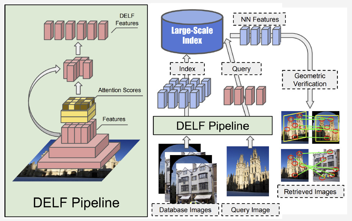
How does landmark recognition work? We have a bank of photos and an input image, and we want to know whether it shows a landmark or not. By running DELF network of all photos, corresponding features for the database and the input image can be obtained. Then we perform a search by the nearest-neighbor method and obtain candidate images with features at the output. We use geometrical verification to match the features: if successful, we conclude that the picture shows a landmark.
Convolutional neural network
Pre-training is crucial for Deep Learning. So we used a database of scenes to pre-train our neural network. Why this way? A scene is a multiple object which comprises a large number of other objects. Landmark is an instance of a scene. By pre-training the model with such a database, we can give it an idea of some low-level features which can be then generalized for successful landmark recognition.
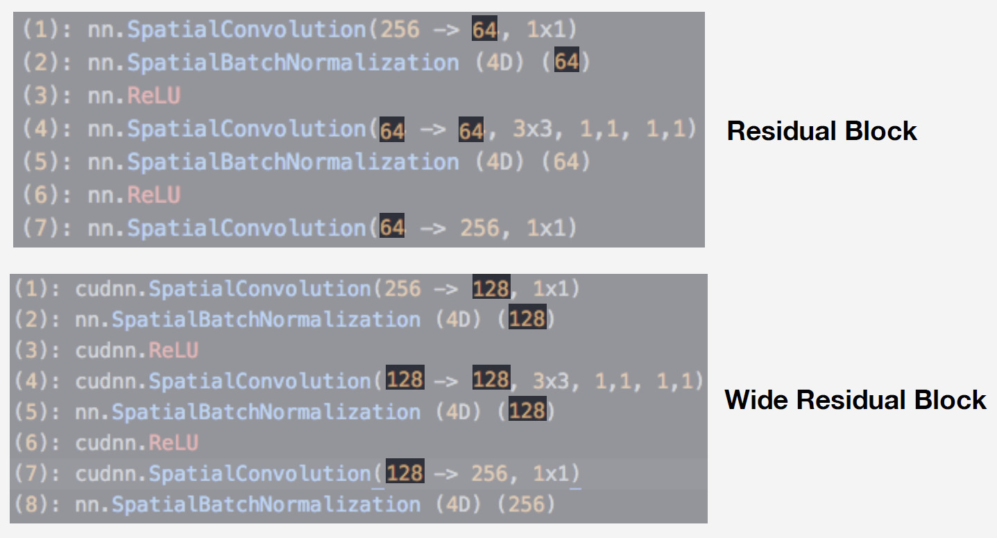
We used a neural network from the Residual network family as the model. The critical difference of such networks is that they use a residual block that includes skip connection which allows a signal to jump over layers with weights and pass freely. Such architecture makes it possible to train deep networks with a high level of quality and control vanishing gradient effect, which is essential for training.
Our model is Wide ResNet-50-2, a version of ResNet-50 where the number of convolutions in the internal bottleneck block is doubled.
The network performs very well. We tested it with our scene database, and here are the results:
| Model |
Top 1 err |
Top 5 err |
|---|---|---|
| ResNet-50 |
46.1 % |
15.7 % |
| ResNet-200 |
42.6 % |
12.9 % |
| SE-ResNext-101 |
42 % |
12.1 % |
| WRN-50-2 (fast!) |
41.8 % |
11.8 % |
Wide ResNet worked nearly twice as fast as ResNet-200. After all, it is running speed that is crucial for production. Given all these considerations, we chose Wide ResNet-50-2 as our main neural network.
Training
We need a loss function to train our network. We decided to use metric learning approach to pick it: a neural network is trained so that items of the same class flock to one cluster, while clusters for different classes are to be spaced apart as much as possible. For landmarks, we used Center loss which pulls elements of one class towards some center. An important feature of this approach is that it does not require negative sampling, which becomes a rather difficult thing to do at later epochs.

Remember that we have n classes of landmarks and one more “non-landmark” class for which Center loss is not used. We imply that a landmark is one and the same object, and it has structure, so it makes sense to determine its center. As to non-landmark, it can refer to whatever, so it makes no sense to determine center for it.
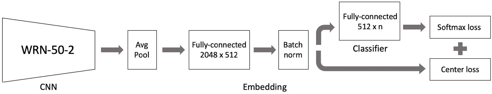
We then put all this together, and there is our model for training. It comprises three major parts:
- Wide ResNet 50-2 convolutional neural network pre-trained with a database of scenes;
- Embedding part comprising a fully connected layer and Batch norm layer;
- Classifier which is a fully connected layer, followed by a pair comprised of Softmax loss and Centre loss.
As you remember, our database is split into 4 parts by region. We use these 4 parts in a curriculum learning paradigm. We have a current dataset, and at each stage of learning, we add another part of the world to obtain a new dataset for training.
The model comprises three parts, and we use a specific learning rate for each one in the training process. This is required for the network to be able both to learn landmarks from a new dataset part we have added and to remember data already learned. Many experiments proved this approach to be the most efficient.
So, we have trained our model. Now we need to realize how it works. Let us use class activation map to find the part of the image to which our neural network reacts most readily. The picture below shows input images in the first row, and the same images overlaid with class activation map from the network we have trained at the previous step are shown in the second row.
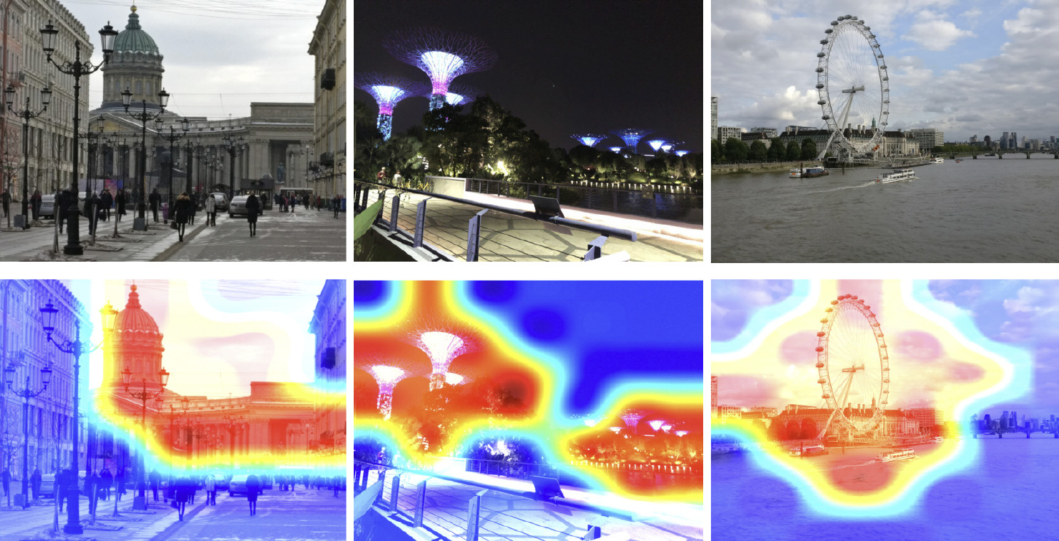
Heat map shows which parts of the image are attended more by the network. As shown by class activation map, our neural network has learned the concept of landmark successfully.
Inference
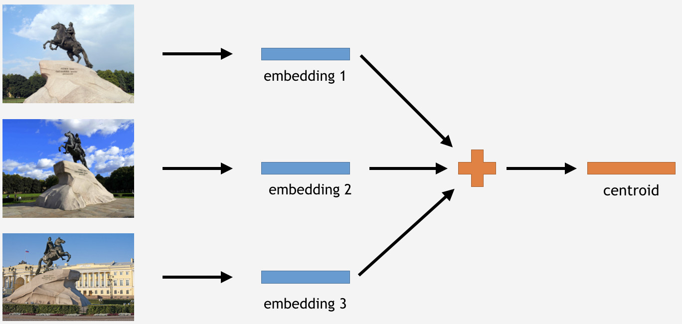
Now we need to use this knowledge somehow to get things done. Since we have used Center loss for training, in the case of inference, it appears to be quite logical to determine centroids for landmarks too.
To do this, we take a part of images from the training set for some landmark, say, the Bronze Horseman in Saint Petersburg. Then we have them processed by the network, obtain embeddings, average out, and derive a centroid.
However, here is a question: how many centroids per landmark it makes sense to derive? Initially, it appeared to be clear and logical to say: one centroid. Not exactly, as it turned out. We initially decided to make a single centroid too, and the result was not bad. So why several centroids?
First, the data we have is not so clean. Though we have cleaned the dataset, we removed only obvious waste data. However, there still could be images not obviously waste but adversely affecting the result.
For example, I have a landmark class Winter Palace in Saint Petersburg. I want to derive a centroid for it. However, its dataset includes some photos with Palace Square and General Headquarters arch, because these objects are close to each other. If the centroid is to be determined for all images, the result will be not so stable. What we need to do is to cluster somehow their embeddings derived from the neural network, take only the centroid that deals with the Winter Palace, and average out using the resulting data.
Second, photographs might have been taken from different angles.
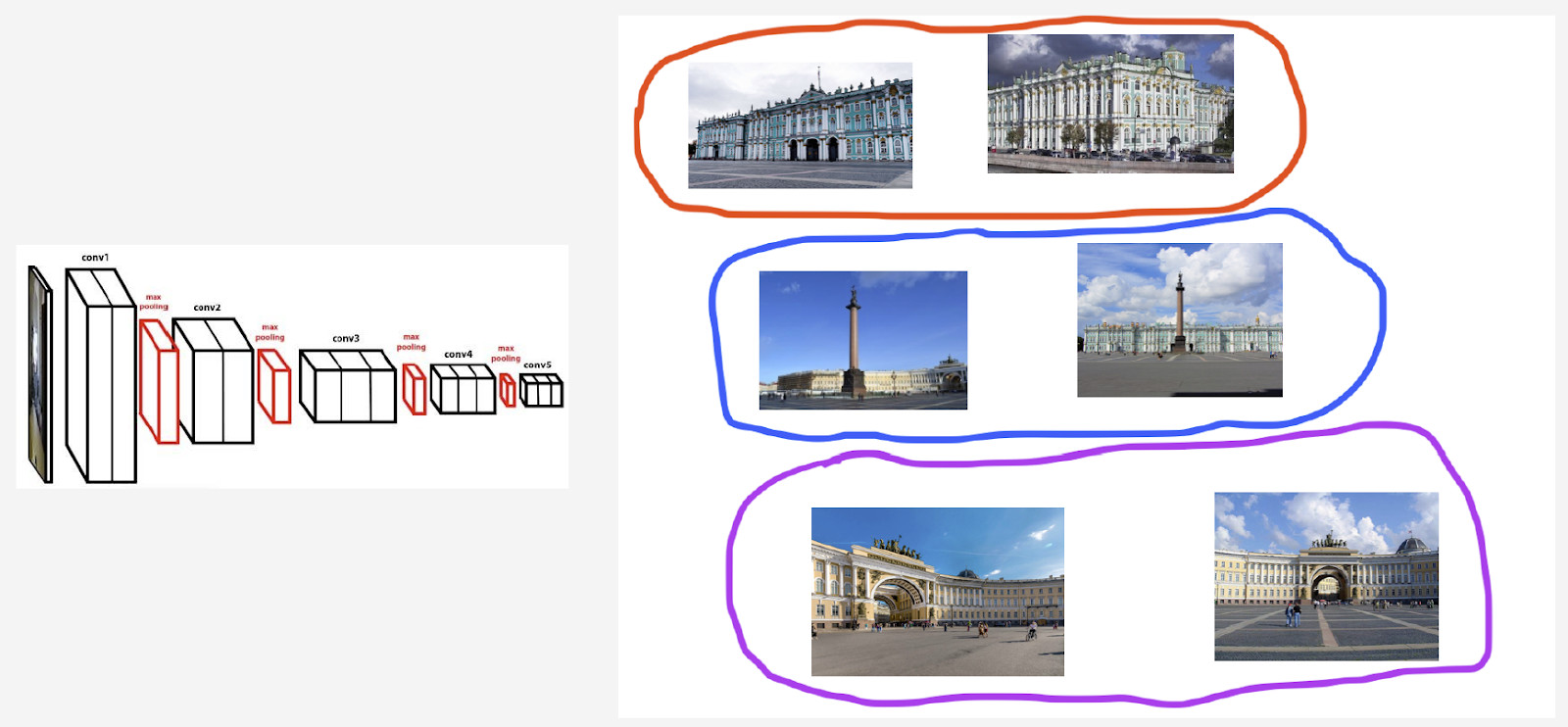
Here is an example of such behavior illustrated with the Belfry of Bruges. Two centroids have been derived for it. In the top row in the image, there are those photos which are closer to the first centroid, and in the second row — the ones that are closer to the second centroid.
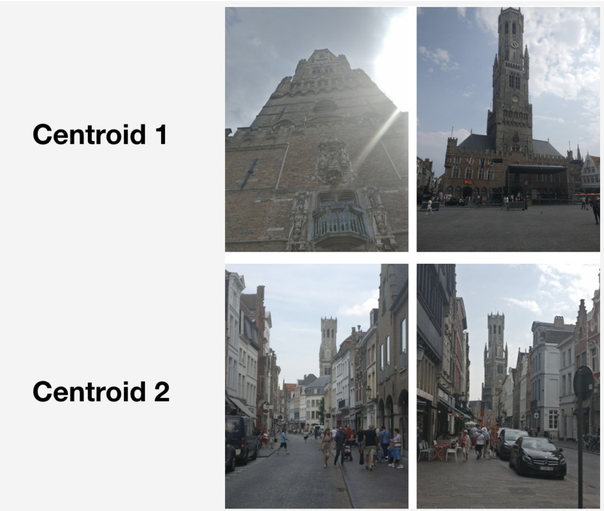
The first centroid deals with more “grand” photographs which were taken at the marketplace in Bruges at short range. The second centroid deals with photographs taken from a distance in particular streets.
As it turns out, by deriving several centroids per landmark class, we can reflect on inference different camera angles for that landmark.
So, how do we obtain those sets for deriving centroids? We apply hierarchical clustering (complete link) to datasets for each landmark. We use it to find valid clusters from which centroids are to be derived. By valid clusters we mean those comprising at least 50 photographs as a result of clustering. The other clusters are rejected. As a result, we obtained around 20 % of landmarks with more than one centroid.
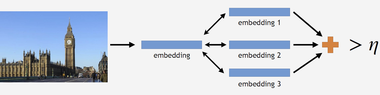
Now to inference. It is obtained in two steps: firstly, we feed the input image to our convolutional neural network and obtain embedding, and then match the embedding with centroids using dot product. If images have geo data, we restrict the search to centroids, which refer to landmarks located within a 1x1 km square from the image location. This enables a more accurate search and a lower threshold for subsequent matching. If the resulting distance exceeds the threshold which is a parameter of the algorithm, then we conclude that a photo has a landmark with the maximum dot product value. If it is less, then it is a non-landmark photo.
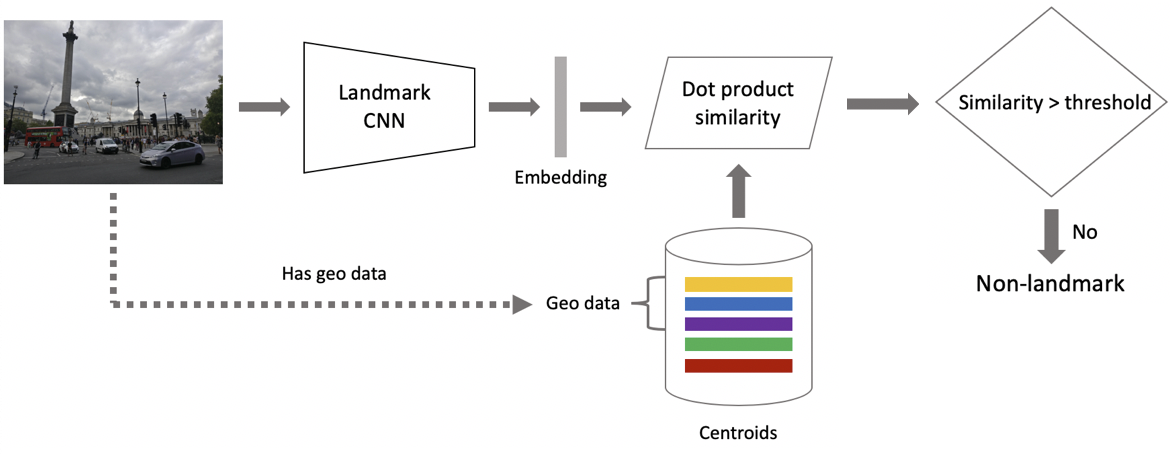
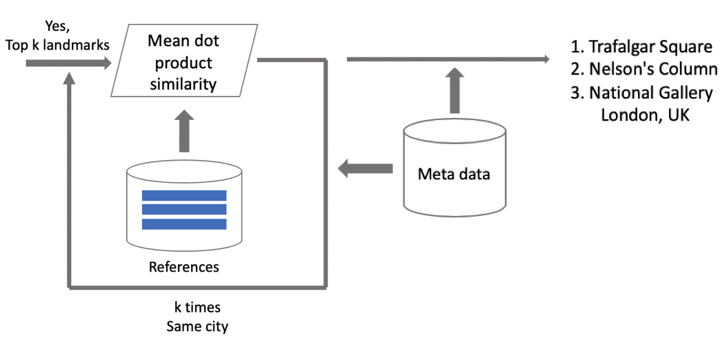
Suppose that a photo has a landmark. If we have geo data, then we use it and derive an answer. If geo data is unavailable, then we run an additional check. When we were cleaning the dataset, we made a set of reference images for each class. We can determine embeddings for them, and then obtain average distance from them to the embedding of the query image. If it exceeds some threshold, then verification is passed, and we bring in metadata and derive a result. It is important to note that we can run this procedure for several landmarks which have been found in an image.
Results of tests
We compared our model with DELF, for which we took parameters with which it would show the best performance in our test. The results are nearly identical.
| Model |
Landmark |
Non-landmark |
|---|---|---|
| Our model |
80 % |
99 % |
| DELF |
80.1 % |
99 % |
Then we classified landmarks into two types: frequent (over 100 photographs in the database), which accounted for 87 % of all landmarks in the test, and rare. Our model works well with the frequent ones: 85.3 % precision. With rare landmarks, we had 46 % which was also not bad at all, meaning that our approach worked fairly well even with few data.
| Type |
Precision |
Share of the total number |
|---|---|---|
| Frequent |
85.3 % |
87 % |
| Rare |
46 % |
13 % |
Then we ran A/B test with user photos. As a result, cloud space purchase conversion rate grew by 10 %, mobile app uninstall conversion rate reduced by 3 %, and the number of album views increased by 13 %.
Let us compare our speed to DELF’s. With GPU, DELF requires 7 network runs because it uses 7 image scales, while our approach uses only 1. With CPU, DELF uses a longer search by the nearest-neighbor method and a very long geometrical verification. In the end, our method was 15 times faster with CPU. Our approach shows higher speed in both cases, which is crucial for production.
Results: memories from vacation
At the beginning of this article, I mentioned a solution for scrolling and finding desired landmark pictures. Here it is.
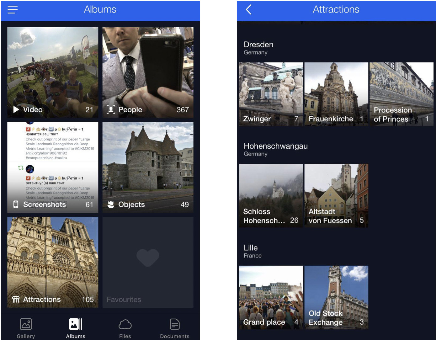
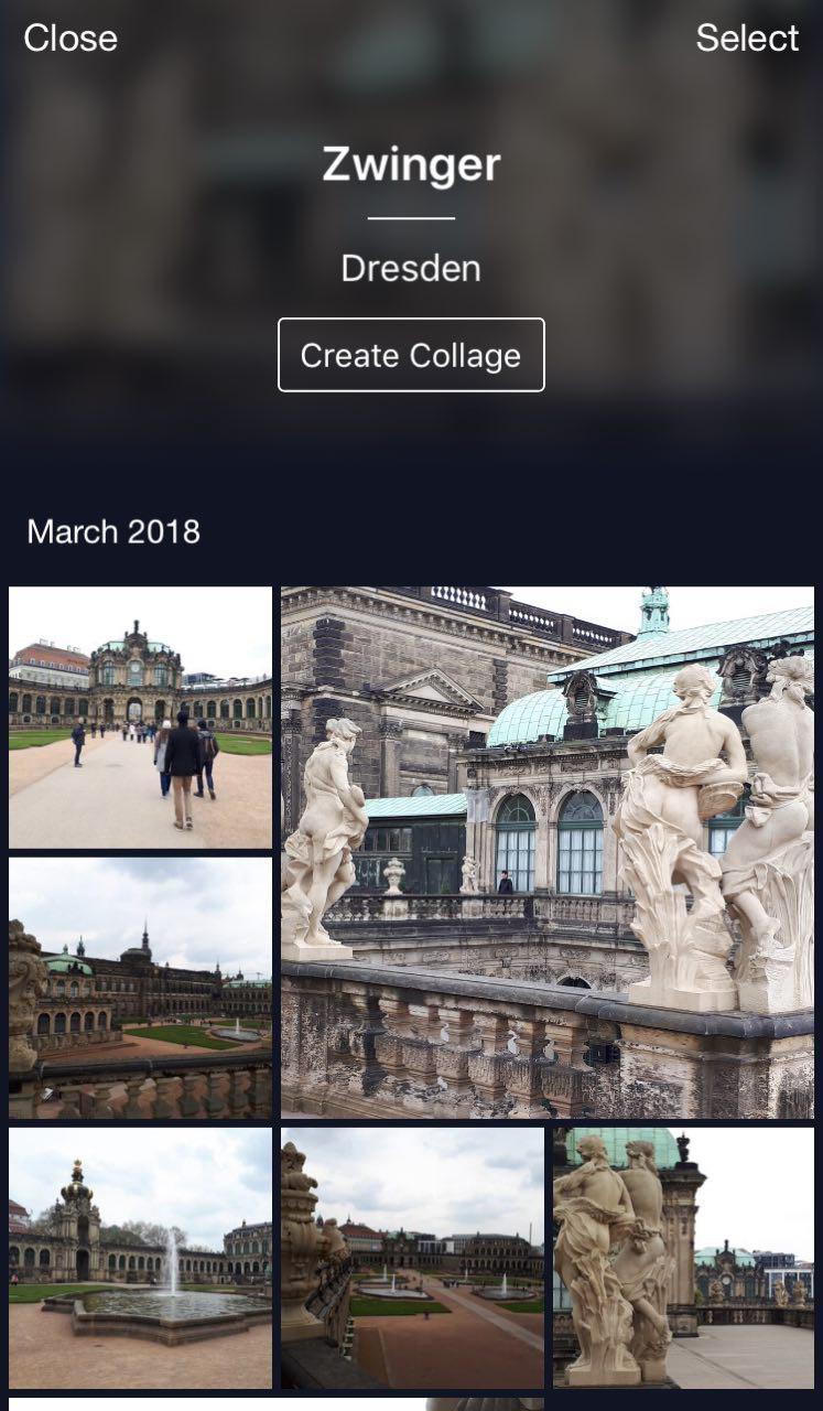
This is my cloud where all photos are classified into albums. There are albums “People”, “Objects”, and “Attractions”. In Attractions album, the landmarks are classified into albums that are grouped by city. A click on Dresdner Zwinger opens an album with photos of this landmark only.
A handy feature: you can go on vacation, take some photos and store them in your cloud. Later, when you wish to upload them to Instagram or share with friends and family, you won’t have to search and pick too long — the desired photos will be available in just a few clicks.
Conclusions
Let me remind you of the key features of our solution.
- Semi-automatic database cleaning. A bit of manual work is required for initial mapping, and then the neural network will do the rest. This allows for cleaning new data quickly and using it to retrain the model.
- We use deep convolutional neural networks and deep metric learning which allows us to learn structure in classes efficiently.
- We have used curriculum learning, i.e. training in parts, as training paradigm. This approach has been very helpful to us. We use several centroids on inference, which allow using cleaner data and find different views of landmarks.
It might seem that object recognition is a trivial task. However, exploring real-life user needs, we find new challenges like landmark recognition. This technique makes it possible to tell people something new about the world using neural networks. It is very encouraging and motivating!
