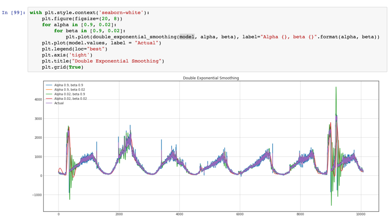
This is a short article about understanding time series and main characteristics behind that.
We have time-series data with daily and weekly regularity. We want to find the way how to model this data in an optimal way.
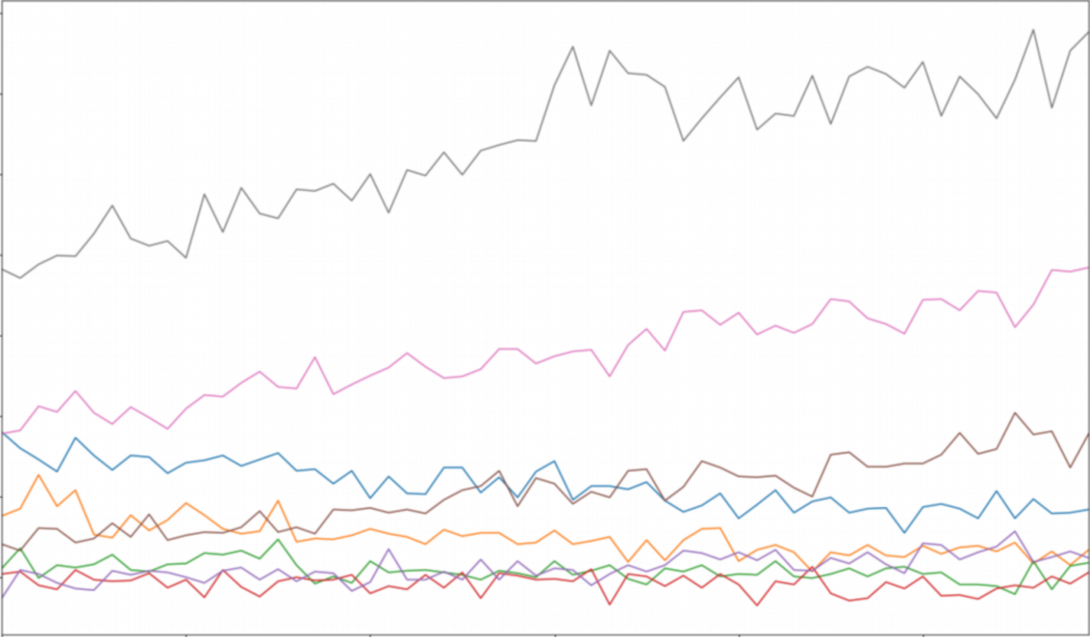
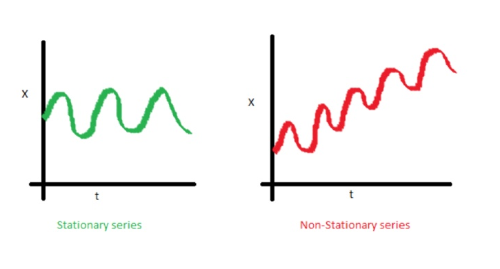
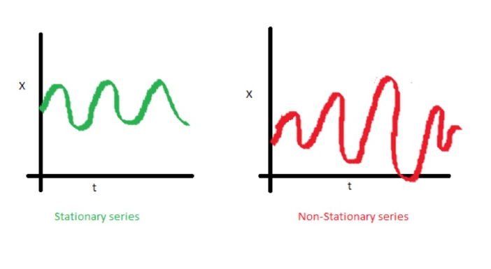
One of the important characteristics of time series is stationarity.
In mathematics and statistics, a stationary process (a.k.a. a strict(ly) stationary process or strong(ly) stationary process) is a stochastic process whose joint probability distribution does not change when shifted in time.
Consequently, parameters such as mean and variance, if they are present, also do not change over time. Since stationarity is an assumption underlying many statistical procedures used in time series analysis, non-stationary data is often transformed to become stationary.
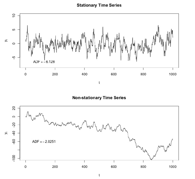
The most common cause of violation of stationarity are trends in mean, which can be due either to the presence of a unit root or of a deterministic trend. In the former case of a unit root, stochastic shocks have permanent effects and the process is not mean-reverting. In the latter case of a deterministic trend, the process is called a trend stationary process, and stochastic shocks have only transitory effects which are mean-reverting (i.e., the mean returns to its long-term average, which changes deterministic over time according to the trend).
Trend line
Dispersion
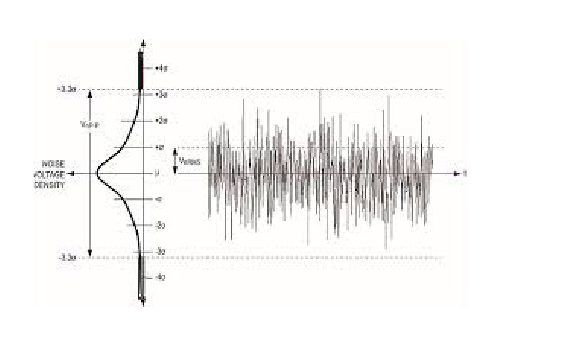
White noise is a stochastic stationary process which can be described using two parameters: mean and dispersion(variance). In discrete time, white noise is a discrete signal whose samples are regarded as a sequence of serially uncorrelated random variables with zero mean and finite variance.
If we make projection onto axis y we can see normal distribution. White noise is a gaussian process in time.
In probability theory, the normal (or Gaussian) distribution is a very common continuous probability distribution. Normal distributions are important in statistics and are often used in the natural and social sciences to represent real-valued random variables whose distributions are not known. The normal distribution is useful because of the central limit theorem. In its most general form, under some conditions (which include finite variance), it states that averages of samples of observations of random variables independently drawn from independent distributions converge in distribution to the normal, that is, become normally distributed when the number of observations is sufficiently large. Physical quantities that are expected to be the sum of many independent processes (such as measurement errors) often have distributions that are nearly normal. Moreover, many results and methods (such as propagation of uncertainty and least squares parameter fitting) can be derived analytically in explicit form when the relevant variables are normally distributed.
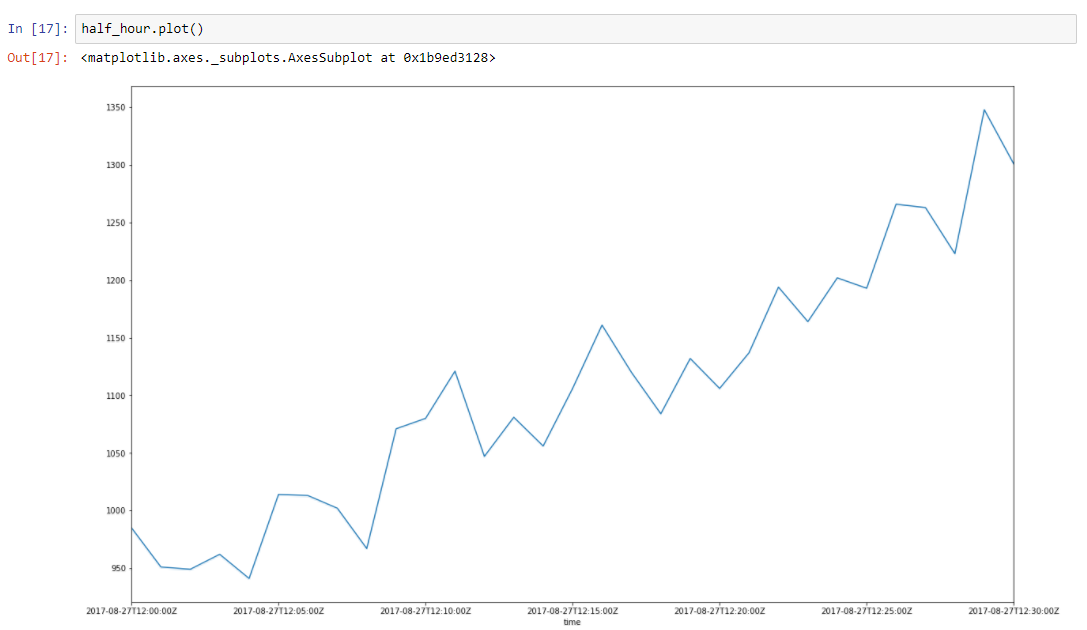
Assume that our data has some trend. Spikes around it is due to a lot of random factors, that affects our data. For example amount of served requests is described using this approach very well. Garbage collection, cache misses, paging by OS, a lot of things affects particular time of served response. Lets take half an hour slice from our data, from 2017–08–27 12:00 till 12:30. We can see that this data has a trend, and some oscillations
Let’s build regression line for defining slope of this trend line.
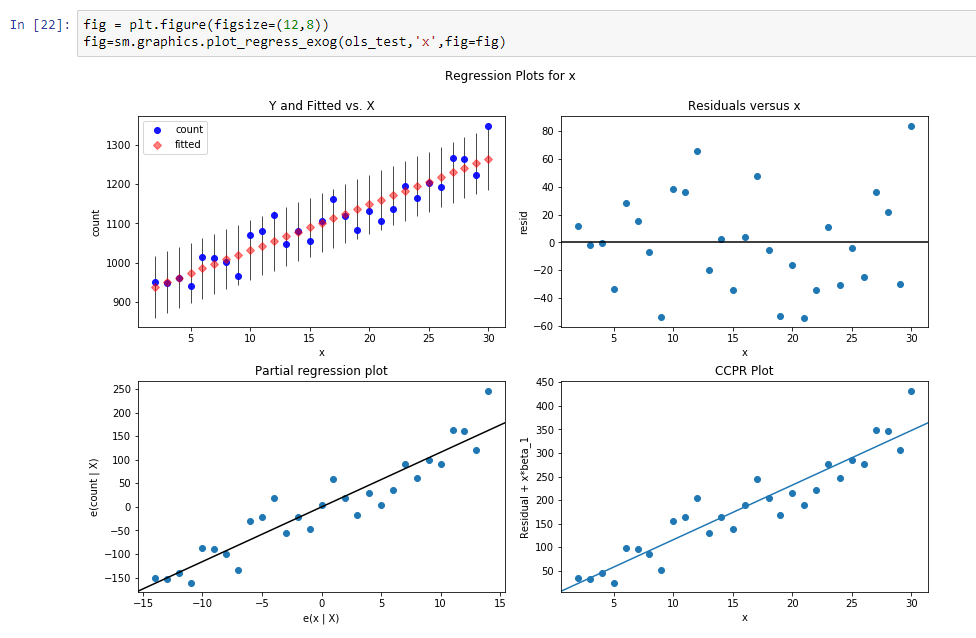
Results of this regression are:
const 916.269951
dy/dx 11.599507
Results means, that const is a level for this trend line, and dy/dx is a slope line which defines how fast level grows according time.
So actually we reduce dimension of data from 31 parameters to 2 parameters. If we subtract from our initial data our regression function values we will see process, that looks like stationary stochastic process.
So after subtraction we can see that trend is disappeared and we can assume that process is stochastic in this range. But how we can be sure.
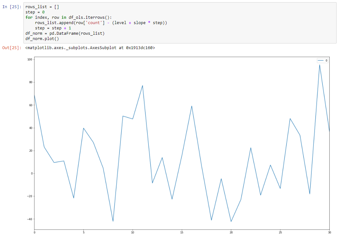
Let’s make Dickey–Fuller test.
Dickey–Fuller tests null hypothesis that time series has root and is stationary as well or rejects this hypothesis. If we make Dickey-Fuller test on our initial slice, we will get
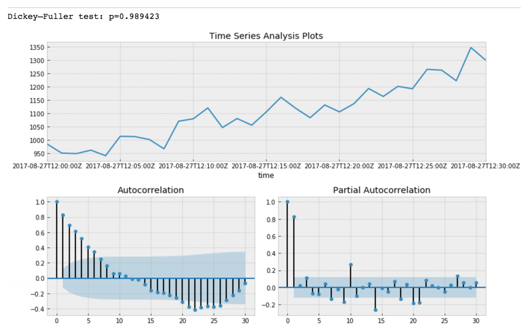
Value of Dickey-Fuller Test rejects null hypothesis with a strong confidence. Thus our time series slice is a non-stationary one. And we can see that Autocorrelation Function shows hidden autocorrelations.
After subtraction of our regression model from initial data.
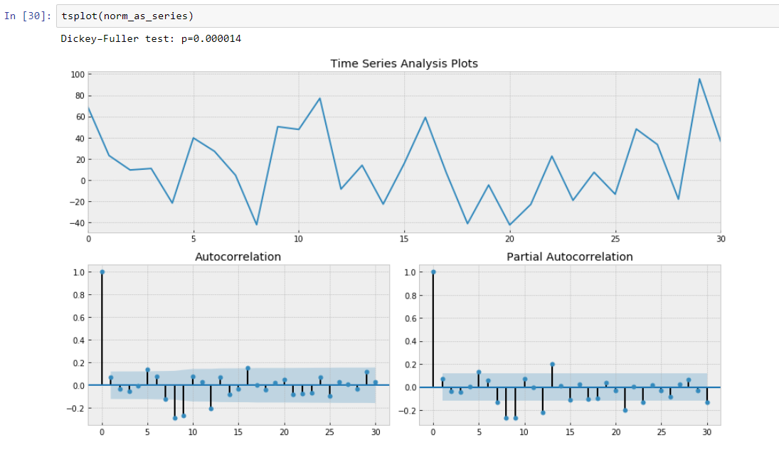
Here we can see that Dickey-Fuller Test value is really small and do not reject a null hypothesis about non stationarity of our time series slice. Also autocorrelation function looks well.
Thus we have made some transformation of our data and we can rotate our data according our slope of our trend line.
Segmented regression, also known as piecewise regression or “broken-stick regression”, is a method in regression analysis in which the independent variable is partitioned into intervals and a separate line segment is fit to each interval. Segmented regression analysis can also be performed on multivariate data by partitioning the various independent variables. Segmented regression is useful when the independent variables, clustered into different groups, exhibit different relationships between the variables in these regions. The boundaries between the segments are breakpoints.
Actually our slope is a discrete derivative of our non stationary time series due to the constant interval of our metric points we can not to take in account dx. Hence we can approximate our data as piecewise function which computed using discrete derivatives of time series regression trends.
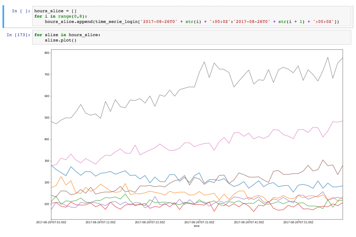
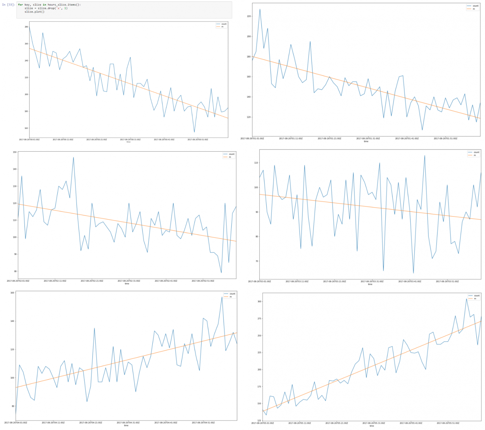
Above is a data slice from 26–08–2017 00.00 till 08.00
It looks like there is a linear autocorrelation for every slice and if we find a regression line for every slice we can build model of our time slices using assumptions that we made.
As a result we will have data which is described using minimal amount of parameters which is favorable due to a better generalization. Vapnik — Chervonenkis dimension should be as small as possible for a good generalization.
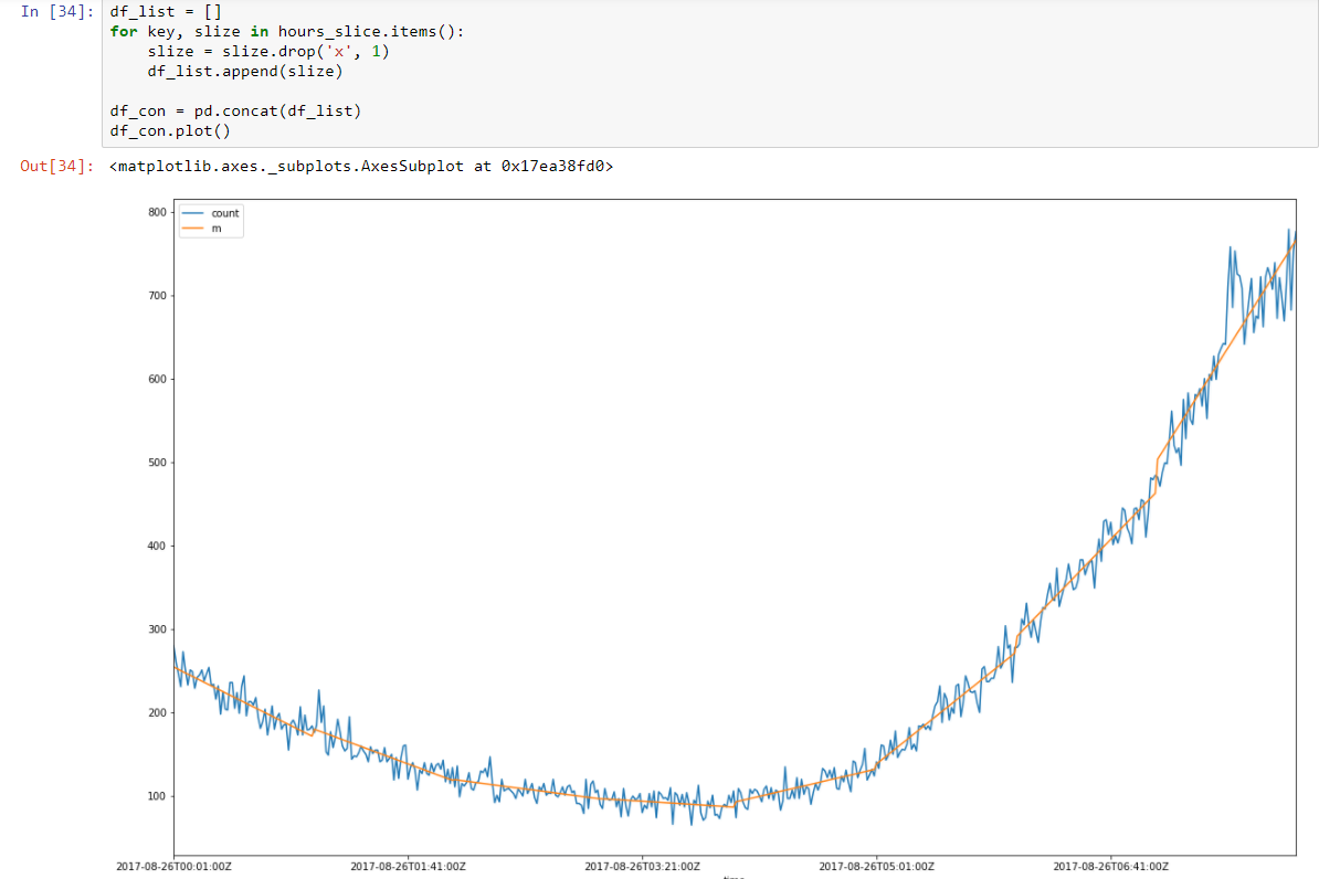
Putting together all 8 hour slices
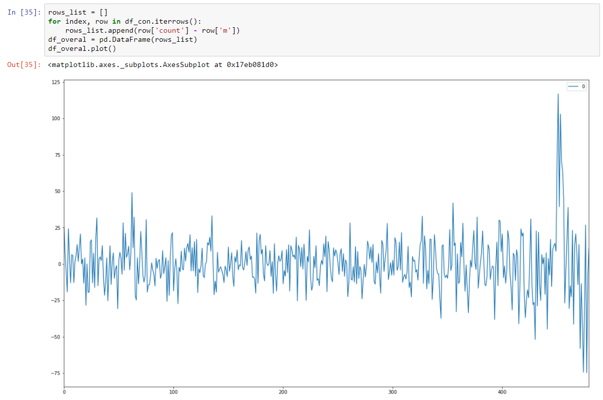
And make it stationary stochastic by subtracting regression model.
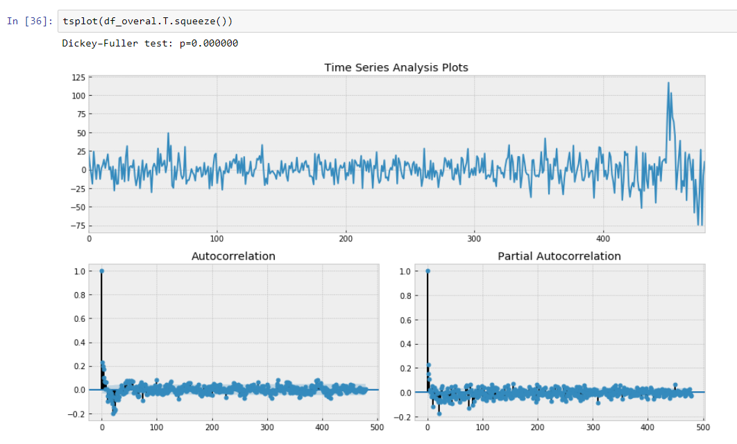
And our Dickey-Fuller test on stationary is showing with a strong confidence that we transformed our data to stationary series.
So we have a prediction model which describes our time series data. We have reduced dimensionality of our data 15/30 times smaller!
Actually we should return mean of our model’s prediction and transform it back using level and slope for a particular slice. It will minimize sum of squared errors for our models prediction.
But we should store variance as well because increase in variance could lead to the presence of new unknown factors and as we know from domain knowledge it is so.
So rapid changing in variance should be alerted as well.
We want to use ARIMA model as well but more general approach is better, and we plan to compare this model, and standard ARIMA for better results. Let see our time series (Green are variance bursts on outliers)

Problem statement
We have time-series data with daily and weekly regularity. We want to find the way how to model this data in an optimal way.

Analyzing time series
One of the important characteristics of time series is stationarity.
In mathematics and statistics, a stationary process (a.k.a. a strict(ly) stationary process or strong(ly) stationary process) is a stochastic process whose joint probability distribution does not change when shifted in time.
Consequently, parameters such as mean and variance, if they are present, also do not change over time. Since stationarity is an assumption underlying many statistical procedures used in time series analysis, non-stationary data is often transformed to become stationary.
The most common cause of violation of stationarity are trends in mean, which can be due either to the presence of a unit root or of a deterministic trend. In the former case of a unit root, stochastic shocks have permanent effects and the process is not mean-reverting. In the latter case of a deterministic trend, the process is called a trend stationary process, and stochastic shocks have only transitory effects which are mean-reverting (i.e., the mean returns to its long-term average, which changes deterministic over time according to the trend).
Examples of stationary vs non-stationary processes
Trend line

Dispersion


White noise is a stochastic stationary process which can be described using two parameters: mean and dispersion(variance). In discrete time, white noise is a discrete signal whose samples are regarded as a sequence of serially uncorrelated random variables with zero mean and finite variance.
If we make projection onto axis y we can see normal distribution. White noise is a gaussian process in time.

In probability theory, the normal (or Gaussian) distribution is a very common continuous probability distribution. Normal distributions are important in statistics and are often used in the natural and social sciences to represent real-valued random variables whose distributions are not known. The normal distribution is useful because of the central limit theorem. In its most general form, under some conditions (which include finite variance), it states that averages of samples of observations of random variables independently drawn from independent distributions converge in distribution to the normal, that is, become normally distributed when the number of observations is sufficiently large. Physical quantities that are expected to be the sum of many independent processes (such as measurement errors) often have distributions that are nearly normal. Moreover, many results and methods (such as propagation of uncertainty and least squares parameter fitting) can be derived analytically in explicit form when the relevant variables are normally distributed.
Assume that our data has some trend. Spikes around it is due to a lot of random factors, that affects our data. For example amount of served requests is described using this approach very well. Garbage collection, cache misses, paging by OS, a lot of things affects particular time of served response. Lets take half an hour slice from our data, from 2017–08–27 12:00 till 12:30. We can see that this data has a trend, and some oscillations

Let’s build regression line for defining slope of this trend line.

Results of this regression are:
const 916.269951
dy/dx 11.599507
Results means, that const is a level for this trend line, and dy/dx is a slope line which defines how fast level grows according time.
So actually we reduce dimension of data from 31 parameters to 2 parameters. If we subtract from our initial data our regression function values we will see process, that looks like stationary stochastic process.
So after subtraction we can see that trend is disappeared and we can assume that process is stochastic in this range. But how we can be sure.

Let’s make Dickey–Fuller test.
Dickey–Fuller tests null hypothesis that time series has root and is stationary as well or rejects this hypothesis. If we make Dickey-Fuller test on our initial slice, we will get

Value of Dickey-Fuller Test rejects null hypothesis with a strong confidence. Thus our time series slice is a non-stationary one. And we can see that Autocorrelation Function shows hidden autocorrelations.
After subtraction of our regression model from initial data.

Here we can see that Dickey-Fuller Test value is really small and do not reject a null hypothesis about non stationarity of our time series slice. Also autocorrelation function looks well.
Thus we have made some transformation of our data and we can rotate our data according our slope of our trend line.
Segmented Regression of the Data
Segmented regression, also known as piecewise regression or “broken-stick regression”, is a method in regression analysis in which the independent variable is partitioned into intervals and a separate line segment is fit to each interval. Segmented regression analysis can also be performed on multivariate data by partitioning the various independent variables. Segmented regression is useful when the independent variables, clustered into different groups, exhibit different relationships between the variables in these regions. The boundaries between the segments are breakpoints.
Actually our slope is a discrete derivative of our non stationary time series due to the constant interval of our metric points we can not to take in account dx. Hence we can approximate our data as piecewise function which computed using discrete derivatives of time series regression trends.

Above is a data slice from 26–08–2017 00.00 till 08.00
It looks like there is a linear autocorrelation for every slice and if we find a regression line for every slice we can build model of our time slices using assumptions that we made.
As a result we will have data which is described using minimal amount of parameters which is favorable due to a better generalization. Vapnik — Chervonenkis dimension should be as small as possible for a good generalization.
In Vapnik–Chervonenkis theory, the VC dimension (for Vapnik–Chervonenkis dimension) is a measure of the capacity (complexity, expressive power, richness, or flexibility) of a space of functions that can be learned by a statistical classification algorithm. It is defined as the cardinality of the largest set of points that the algorithm can shatter. It was originally defined by Vladimir Vapnik and Alexey Chervonenkis.So as a result we have approximated our hour slices using segmented regression.
Formally, the capacity of a classification model is related to how complicated it can be. For example, consider the thresholding of a high-degree polynomial: if the polynomial evaluates above zero, that point is classified as positive, otherwise as negative. A high-degree polynomial can be wiggly, so it can fit a given set of training points well. But one can expect that the classifier will make errors on other points, because it is too wiggly. Such a polynomial has a high capacity. A much simpler alternative is to threshold a linear function. This function may not fit the training set well, because it has a low capacity.

Putting together all 8 hour slices

And make it stationary stochastic by subtracting regression model.

And our Dickey-Fuller test on stationary is showing with a strong confidence that we transformed our data to stationary series.

So we have a prediction model which describes our time series data. We have reduced dimensionality of our data 15/30 times smaller!
Actually we should return mean of our model’s prediction and transform it back using level and slope for a particular slice. It will minimize sum of squared errors for our models prediction.
But we should store variance as well because increase in variance could lead to the presence of new unknown factors and as we know from domain knowledge it is so.
So rapid changing in variance should be alerted as well.
We want to use ARIMA model as well but more general approach is better, and we plan to compare this model, and standard ARIMA for better results. Let see our time series (Green are variance bursts on outliers)
