What is the best tool to use for drawing vector pictures? For me and probably for many others, the answer is pretty obvious: Illustrator, or, maybe, Inkscape. At least that's what I thought when I was asked to draw about eight hundred diagrams for a physics textbook. Nothing exceptional, just a bunch of black and white illustrations with spheres, springs, pulleys, lenses and so on. By that time it was already known that the book was going to be made in LaTeX and I was given a number of MS Word documents with embedded images. Some of them were scanned pictures from other books, some were pencil drawings. Picturing days and nights of inkscaping this stuff made me feel dizzy, so soon I found myself fantasizing about a more automated solution. For some reason MetaPost became the focus of these fantasies.
The main advantage of using MetaPost (or similar) solution is that every picture can be a sort of function of several variables. Such a picture can be quickly adjusted for any unforeseen circumstances of the layout, without disrupting important internal relationships of the illustration (something I was really concerned about), which is not easily achieved with more traditional tools. Also, recurring elements, all these spheres and springs, can be made more visually interesting than conventional tools would allow with the same time constraints.
I wanted to make pictures with some kind of hatching, not unlike what you encounter in old books.
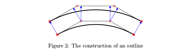
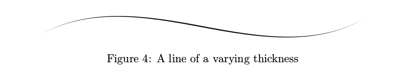
First, I needed to be able to produce some curves of varying thickness. The main complication here is to construct a curve that follows the original curve at a varying distance. I used probably the most primitive working method, which boils down to simply shifting the line segments connecting Bezier curve control points by a given distance, except this distance varies along the curve.
In most cases, it worked OK.
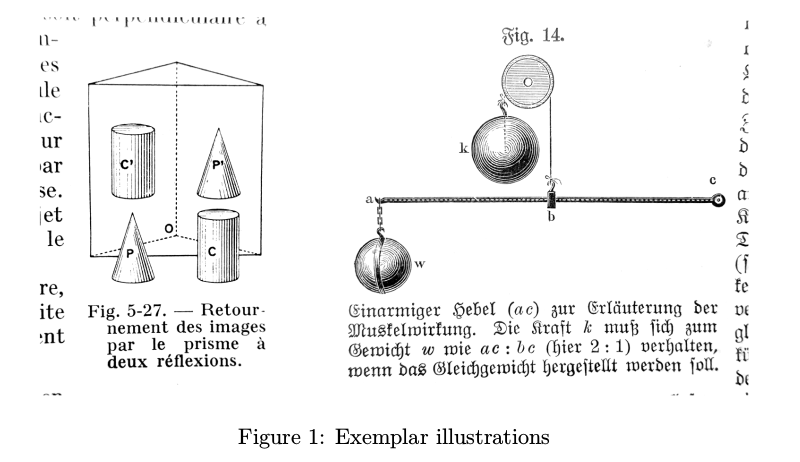
Two outlines can be combined to make a contour line for a variable-thickness stroke.
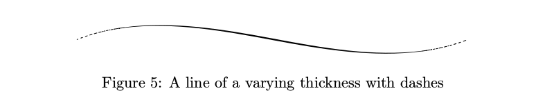
The line thickness should have some lower bound, otherwise, some lines are going to be too thin to be properly printed and this doesn't look great. One of the options (the one I chose) is to make the lines which are too thin dashed, so that the total amount of ink per unit length remains approximately the same as in the intended thinner line. In other words, instead of reducing the amount of ink on the sides of the line, the algorithm takes some ink from the line itself.
Once you have working variable-thickness lines, you can draw spheres. A sphere can be depicted as a series of concentric circles with the line thicknesses varying according to the output of a function that calculates the lightness of a particular point on the sphere.

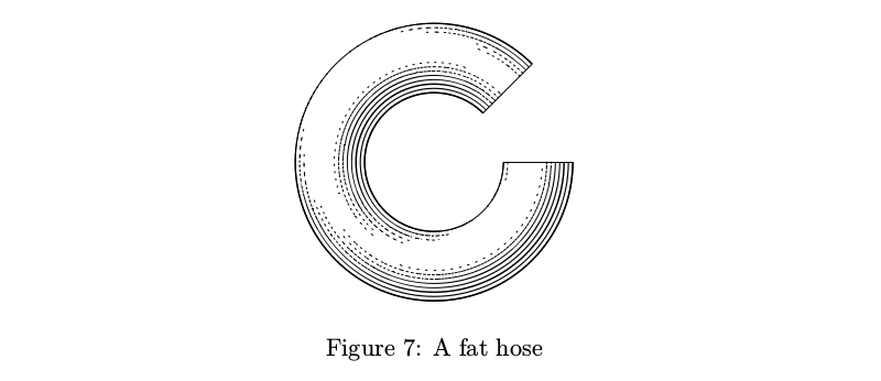
Another convenient construction block is a “tube.” Roughly speaking it is a cylinder which you can bend. So long as the diameter is constant, it's pretty straightforward.
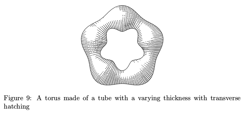
If the diameter isn't constant, things become more complicated: the number of strokes should change according to the tube thickness in order to keep the amount of ink per unit area constant before taking the lights into account.
There are also tubes with transverse hatching. The problem of keeping the amount of ink constant turned out to be even trickier in this case, so ofttimes such tubes look a tad shaggy.
Tubes can be used to construct a wide range of objects: from cones and cylinders to balusters.

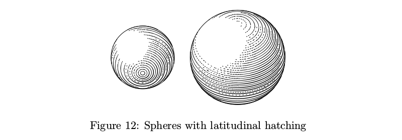
Some constructions which can be made from these primitives are included in the library. For example, the globe is basically a sphere.

However, the hatching here is latitudinal and controlling line density is much more difficult than on the regular spheres with “concentric” hatching, so it's a different kind of sphere.
A weight is a simple construction made from tubes of two types.

There's also a tool to knot the tubes.
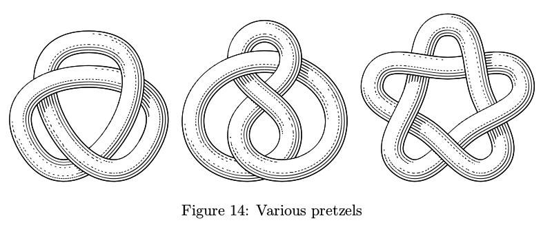
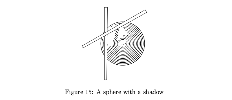
Tubes in knots drop shadows on each other as they should. In theory, this feature can be used in other contexts, but since I had no plans to go deep into the third dimension, the user interface is somewhat lacking and shadows work properly only for some objects.
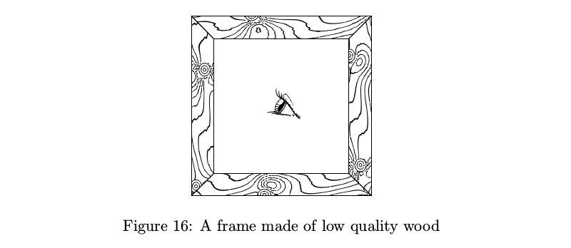
Certainly, you will need a wood texture (update: since the Russian version of this article was published, the first case of this library being used in a real project which I'm aware of has occurred, and it was the wood texture which came in handy, so this ended up not being a joke after all). How twigs and their growth affect the pattern of year rings is a topic for some serious study. The simplest working model I could come up with is as follows: year rings are parallel flat surfaces, distorted by growing twigs; thus the surface is modified by a series of not overly complex “twig functions” in different places and the surface's isolines are taken as the year ring pattern.
The eye from the picture above opens wide or squints a bit and its pupil changes its size too. It may not make any practical sense, but mechanically similar eyes just look boring.

Most of the time the illustrations weren't all that complex, but a more rigorous approach would require solving many of the problems in the textbook to illustrate them correctly. Say, L'Hôpital's pulley problem (it wasn't in that textbook, but anyway): on the rope with the length , suspended at the point
  a pulley is hanging; it's hooked to another rope, suspended at the point
  with the weight
  on its end. The question is: where does the weight go if both the pulley and the ropes weigh nothing? Surprisingly, the solution and the construction for this problem are not that simple. But by playing with several variables you can make the picture look just right for the page while maintaining accuracy.
And what about the textbook? Alas, when almost all the illustrations and the layout were ready, something happened and the textbook was canceled. Maybe because of that, I decided to rewrite most of the functions of the original library from scratch (I chose not to use any of the original code, which, although indirectly, I was paid for) and put it on GitHub. Some things, present in the original library, such as functions for drawing cars and tractors, I didn't include there, some new features, e.g. knots, were added.
It doesn't run quickly: it takes about a minute to produce all the pictures for this article with LuaLaTeX on my laptop with i5-4200U 1.6 GHz. A pseudorandom number generator is used here and there, so no two similar pictures are absolutely identical (that's a feature) and every run produces slightly different pictures. To avoid surprises you can simply set
Many thanks to dr ord and Mikael Sundqvist for their help with the English version of this text.
The main advantage of using MetaPost (or similar) solution is that every picture can be a sort of function of several variables. Such a picture can be quickly adjusted for any unforeseen circumstances of the layout, without disrupting important internal relationships of the illustration (something I was really concerned about), which is not easily achieved with more traditional tools. Also, recurring elements, all these spheres and springs, can be made more visually interesting than conventional tools would allow with the same time constraints.
I wanted to make pictures with some kind of hatching, not unlike what you encounter in old books.
First, I needed to be able to produce some curves of varying thickness. The main complication here is to construct a curve that follows the original curve at a varying distance. I used probably the most primitive working method, which boils down to simply shifting the line segments connecting Bezier curve control points by a given distance, except this distance varies along the curve.
In most cases, it worked OK.
Example code
From here on it is assumed that the library is downloaded and
or LuaLaTeX:
input fiziko.mp; is present in the MetaPost code. The fastest method is to use ConTeXt (then you don't need beginfig and endfig):\starttext
\startMPcode
input fiziko.mp;
% the code goes here
\stopMPcode
\stoptext
or LuaLaTeX:
\documentclass{article}

\usepackage{luamplib}

\begin{document}

\begin{mplibcode}

input fiziko.mp;

% the code goes here

\end{mplibcode}

\end{document}
beginfig(3);

 path p, q; % MetaPost's syntax is reasonably readable, so I'll comment mostly on my stuff

 p := (0,-1/4cm){dir(30)}..(5cm, 0)..{dir(30)}(10cm, 1/4cm);

 q := offsetPath(p)(1cm*sin(offsetPathLength*pi)); % first argument is the path itself, second is a function of the position along this path (offsetPathLength changes from 0 to 1), which determines how far the outline is from the original line

 draw p;

 draw q dashed evenly;

endfig;
Two outlines can be combined to make a contour line for a variable-thickness stroke.
Example code
beginfig(4);

 path p, q[];

 p := (0,-1/4cm){dir(30)}..(5cm, 0)..{dir(30)}(10cm, 1/4cm);

 q1 := offsetPath(p)(1/2pt*(sin(offsetPathLength*pi)**2)); % outline on one side

 q2 := offsetPath(p)(-1/2pt*(sin(offsetPathLength*pi)**2)); % and on the other

 fill q1--reverse(q2)--cycle;

endfig;
The line thickness should have some lower bound, otherwise, some lines are going to be too thin to be properly printed and this doesn't look great. One of the options (the one I chose) is to make the lines which are too thin dashed, so that the total amount of ink per unit length remains approximately the same as in the intended thinner line. In other words, instead of reducing the amount of ink on the sides of the line, the algorithm takes some ink from the line itself.
Example code
beginfig(5);

 path p;

 p := (0,-1/4cm){dir(30)}..(5cm, 0)..{dir(30)}(10cm, 1/4cm);

 draw brush(p)(1pt*(sin(offsetPathLength*pi)**2)); % the arguments are the same as for the outline

endfig;
Once you have working variable-thickness lines, you can draw spheres. A sphere can be depicted as a series of concentric circles with the line thicknesses varying according to the output of a function that calculates the lightness of a particular point on the sphere.
Example code
beginfig(6);

 draw sphere.c(1.2cm);

 draw sphere.c(2.4cm) shifted (2cm, 0);

endfig;
Another convenient construction block is a “tube.” Roughly speaking it is a cylinder which you can bend. So long as the diameter is constant, it's pretty straightforward.
Example code
beginfig(7);

 path p;

 p := subpath (1,8) of fullcircle scaled 3cm;

 draw tube.l(p)(1/2cm); % arguments are the path itself and the tube radius

endfig;
If the diameter isn't constant, things become more complicated: the number of strokes should change according to the tube thickness in order to keep the amount of ink per unit area constant before taking the lights into account.
Example code
beginfig(8);

 path p;

 p := pathSubdivide(fullcircle, 2) scaled 3cm; % this thing splits every segment between the points of a path (here—fullcircle) into several parts (here—2)

 draw tube.l(p)(1/2cm + 1/6cm*sin(offsetPathLength*10pi));

endfig;
There are also tubes with transverse hatching. The problem of keeping the amount of ink constant turned out to be even trickier in this case, so ofttimes such tubes look a tad shaggy.
Example code
beginfig(9);

 path p;

 p := pathSubdivide(fullcircle, 2) scaled 3cm;

 draw tube.t(p)(1/2cm + 1/6cm*sin(offsetPathLength*10pi));

endfig;
Tubes can be used to construct a wide range of objects: from cones and cylinders to balusters.
Example code
beginfig(10);

 draw tube.l ((0, 0) -- (0, 3cm))((1-offsetPathLength)*1cm) shifted (-3cm, 0); % a very simple cone

 path p;

 p := (-1/2cm, 0) {dir(175)} .. {dir(5)} (-1/2cm, 1/8cm) {dir(120)} .. (-2/5cm, 1/3cm) .. (-1/2cm, 3/4cm) {dir(90)} .. {dir(90)}(-1/4cm, 9/4cm){dir(175)} .. {dir(5)}(-1/4cm, 9/4cm + 1/5cm){dir(90)} .. (-2/5cm, 3cm); % baluster's envelope

 p := pathSubdivide(p, 6);

 draw p -- reverse(p xscaled -1) -- cycle;

 tubeGenerateAlt(p, p xscaled -1, p rotated -90); % a more low-level stuff than tube.t, first two arguments are tube's sides and the third is the envelope. The envelope is basically a flattened out version of the outline, with line length along the x axis and the distance to line at the y. In the case of this baluster, it's simply its side rotated 90 degrees.

endfig;
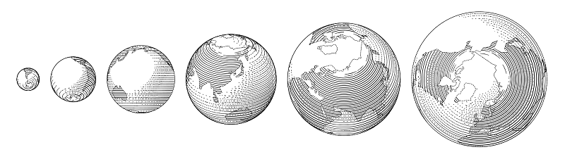
Some constructions which can be made from these primitives are included in the library. For example, the globe is basically a sphere.
Example code
beginfig(11);

 draw globe(1cm, -15, 0) shifted (-6/2cm, 0); % radius, west longitude, north latitude, both decimal

 draw globe(3/2cm, -30.280577, 59.939461);

 draw globe(4/3cm, -140, -30) shifted (10/3cm, 0);

endfig;
However, the hatching here is latitudinal and controlling line density is much more difficult than on the regular spheres with “concentric” hatching, so it's a different kind of sphere.
Example code
beginfig(12);

 draw sphere.l(2cm, -60); % diameter and latitude

 draw sphere.l(3cm, 45) shifted (3cm, 0);

endfig;
A weight is a simple construction made from tubes of two types.
Example code
beginfig(13);

 draw weight.s(1cm); % weight height

 draw weight.s(2cm) shifted (2cm, 0);

endfig;
There's also a tool to knot the tubes.
Example code. For brevity's sake only one knot.
beginfig(14);

 path p;

 p := (dir(90)*4/3cm) {dir(0)} .. tension 3/2 ..(dir(90 + 120)*4/3cm){dir(90 + 30)} .. tension 3/2 ..(dir(90 - 120)*4/3cm){dir(-90 - 30)} .. tension 3/2 .. cycle;

 p := p scaled 6/5;

 addStrandToKnot (primeOne) (p, 1/4cm, "l", "1, -1, 1"); % first, we add a strand of width 1/4cm going along the path p to the knot named primeOne. its intersections along the path go to layers "1, -1, 1" and the type of tube is going to be "l".

 draw knotFromStrands (primeOne); % then the knot is drawn. you can add more than one strand.

endfig;
Tubes in knots drop shadows on each other as they should. In theory, this feature can be used in other contexts, but since I had no plans to go deep into the third dimension, the user interface is somewhat lacking and shadows work properly only for some objects.
Example code
beginfig(15);

 path shadowPath[];

 boolean shadowsEnabled;

 numeric numberOfShadows;

 shadowsEnabled := true; % shadows need to be turned on

 numberOfShadows := 1; % number of shadows should be specified

 shadowPath0 := (-1cm, -2cm) -- (-1cm, 2cm) -- (-1cm +1/6cm, 2cm) -- (-1cm + 1/8cm, -2cm) -- cycle; % shadow-dropping object should be a closed path

 shadowDepth0 := 4/3cm; % it's just this high above the object on which the shadow falls

 shadowPath1 := shadowPath0 rotated -60;

 shadowDepth1 := 4/3cm;

 draw sphere.c(2.4cm); % shadows work ok only with sphere.c and tube.l with constant diameter

 fill shadowPath0 withcolor white;

 draw shadowPath0;

 fill shadowPath1 withcolor white;

 draw shadowPath1;

endfig;
Certainly, you will need a wood texture (update: since the Russian version of this article was published, the first case of this library being used in a real project which I'm aware of has occurred, and it was the wood texture which came in handy, so this ended up not being a joke after all). How twigs and their growth affect the pattern of year rings is a topic for some serious study. The simplest working model I could come up with is as follows: year rings are parallel flat surfaces, distorted by growing twigs; thus the surface is modified by a series of not overly complex “twig functions” in different places and the surface's isolines are taken as the year ring pattern.
Example code
beginfig(16);

 numeric w, b;

 pair A, B, C, D, A', B', C', D';

 w := 4cm;

 b := 1/2cm;

 A := (0, 0);

 A' := (b, b);

 B := (0, w);

 B' := (b, w-b);

 C := (w, w);

 C' := (w-b, w-b);

 D := (w, 0);

 D' := (w-b, b);

 draw woodenThing(A--A'--B'--B--cycle, 0); % a piece of wood inside the A--A'--B'--B--cycle path, with wood grain at 0 degrees

 draw woodenThing(B--B'--C'--C--cycle, 90);

 draw woodenThing(C--C'--D'--D--cycle, 0);

 draw woodenThing(A--A'--D'--D--cycle, 90);

 eyescale := 2/3cm; % scale for the eye

 draw eye(150) shifted 1/2[A,C]; % the eye looks in 150 degree direction

endfig;
The eye from the picture above opens wide or squints a bit and its pupil changes its size too. It may not make any practical sense, but mechanically similar eyes just look boring.
Example code
beginfig(17);

 eyescale := 2/3cm; % 1/2cm by default

 draw eye(0) shifted (0cm, 0);

 draw eye(0) shifted (1cm, 0);

 draw eye(0) shifted (2cm, 0);

 draw eye(0) shifted (3cm, 0);

 draw eye(0) shifted (4cm, 0);

endfig;
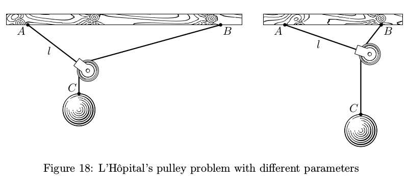
Most of the time the illustrations weren't all that complex, but a more rigorous approach would require solving many of the problems in the textbook to illustrate them correctly. Say, L'Hôpital's pulley problem (it wasn't in that textbook, but anyway): on the rope with the length
, suspended at the point a pulley is hanging; it's hooked to another rope, suspended at the point with the weight on its end. The question is: where does the weight go if both the pulley and the ropes weigh nothing? Surprisingly, the solution and the construction for this problem are not that simple. But by playing with several variables you can make the picture look just right for the page while maintaining accuracy.Example code
vardef lHopitalPulley (expr AB, l, m) = % distance AB between the suspension points of the ropes and their lengths l and m. “Why no units of length?”, you may ask. It's because some calculations inside can cause arithmetic overflow in MetaPost.

 save A, B, C, D, E, o, a, x, y, d, w, h, support;

 image(

 pair A, B, C, D, E, o[];

 path support;

 numeric a, x[], y[], d[], w, h;

 x1 := (l**2 + abs(l)*((sqrt(8)*AB)++l))/4AB; % the solution

 y1 := l+-+x1; % second coordinate is trivial

 y2 := m - ((AB-x1)++y1); % as well as the weight's position

 A := (0, 0);

 B := (AB*cm, 0);

 D := (x1*cm, -y1*cm);

 C := D shifted (0, -y2*cm);

 d1 := 2/3cm; d2 := 1cm; d3 := 5/6d1; % diameters of the pulley, weight and the pulley wheel

 w := 2/3cm; h := 1/3cm; % parameters of the wood block

 o1 := (unitvector(C-D) rotated 90 scaled 1/2d3);

 o2 := (unitvector(D-B) rotated 90 scaled 1/2d3);

 E := whatever [D shifted o1, C shifted o1]

 = whatever [D shifted o2, B shifted o2]; % pulley's center

 a := angle(A-D);

 support := A shifted (-w, 0) -- B shifted (w, 0) -- B shifted (w, h) -- A shifted (-w, h) -- cycle;

 draw woodenThing(support, 0); % wood block everything is suspended from

 draw pulley (d1, a - 90) shifted E; % the pulley

 draw image(

 draw A -- D -- B withpen thickpen;

 draw D -- C withpen thickpen;

 ) maskedWith (pulleyOutline shifted E); % ropes should be covered with the pulley

 draw sphere.c(d2) shifted C shifted (0, -1/2d2); % sphere as a weight

 dotlabel.llft(btex $A$ etex, A);

 dotlabel.lrt(btex $B$ etex, B);

 dotlabel.ulft(btex $C$ etex, C);

 label.llft(btex $l$ etex, 1/2[A, D]);

 )

enddef;

beginfig(18);

 draw lHopitalPulley (6, 2, 11/2); % now you can choose the right parameters

 draw lHopitalPulley (3, 5/2, 3) shifted (8cm, 0);

endfig;
And what about the textbook? Alas, when almost all the illustrations and the layout were ready, something happened and the textbook was canceled. Maybe because of that, I decided to rewrite most of the functions of the original library from scratch (I chose not to use any of the original code, which, although indirectly, I was paid for) and put it on GitHub. Some things, present in the original library, such as functions for drawing cars and tractors, I didn't include there, some new features, e.g. knots, were added.
It doesn't run quickly: it takes about a minute to produce all the pictures for this article with LuaLaTeX on my laptop with i5-4200U 1.6 GHz. A pseudorandom number generator is used here and there, so no two similar pictures are absolutely identical (that's a feature) and every run produces slightly different pictures. To avoid surprises you can simply set
randomseed := some number and enjoy the same results every run.Many thanks to dr ord and Mikael Sundqvist for their help with the English version of this text.
