
This is the concluding part of my article devoted to a statistical analysis of police shootings and criminality among the white and the black population of the United States. In the first part, we talked about the research background, goals, assumptions, and source data; in the second part, we investigated the national use-of-force and crime data and tracked their connection with race.
Let's recall the intermediate inferences that we were able to make from the available data for 2000 — 2018:
- White police victims outnumber black victims in absolute figures.
- Use of lethal force results in an average of 5.9 per one million Black deaths and 2.3 per one million White deaths (Black victim count is 2.6 greater in unit values).
- Year-to-year scatter in Black lethal force fatalities is nearly twice the scatter in White fatalities.
- White fatalities grow continuously from year to year (by 0.1 — 0.2 per million on average), while Black fatalities rolled back to their 2009 level after climaxing in 2011 — 2013.
- Whites commit twice as many offenses as Blacks in absolute numbers, but three times as fewer in per capita numbers (per 1 million population within that race).
- Criminality among Whites grows more or less steadily over the entire period of investigation (doubled over 19 years). Criminality among Blacks also grows, but by leaps and starts; over the entire period, however, the growth factor is also 2, like with Whites.
- Fatal encounters with law enforcement are connected with criminality (number of offenses committed). The correlation though differs between the two races: for Whites, it is almost perfect, for Blacks — far from perfect.
- Lethal force victims grow 'in reply to' criminality growth, generally with a few years' lag (this is more conspicuous in the Black data).
- White offenders tend to meet death from the police a little more frequently than Black offenders.
Today, as I promised, we'll be looking at the geographical distribution of these data across the states, which ought to either confirm or confute the previous conclusions.
However, before we take up geography, let's make a step back and see what happens if we analyze only the most violent offenses instead of 'All Offenses' as the source data for criminality. Many of my readers have pointed out in their comments that this would have been more proper, since 'All Offenses' incorporate those which should not (in practice) be associated with aggressive behavior provoking police shooting, such as petty larceny or selling drugs. I cannot whole-heartedly agree with this reasoning because, as I see it, any offense can arouse or heighten attention from the law enforcement, which in turn may wind up sadly… Still, let's just be curious enough to check!
Assault and Murder Instead of All Offenses
We just need to change one line of code where we form the crime dataset. Replace this line
df_crimes1 = df_crimes1.loc[df_crimes1['Offense'] == 'All Offenses']
with this:
df_crimes1 = df_crimes1.loc[df_crimes1['Offense'].str.contains('Assault|Murder')]
Our new filter now lets through only offenses connected with assault (simple and aggravated) and murder / non-negligent homicide (negligent / justifiable homicide / manslaughter cases are not included).
We leave the rest of the code as it was.
The number of crimes per 1 million population within each race now looks as follows:
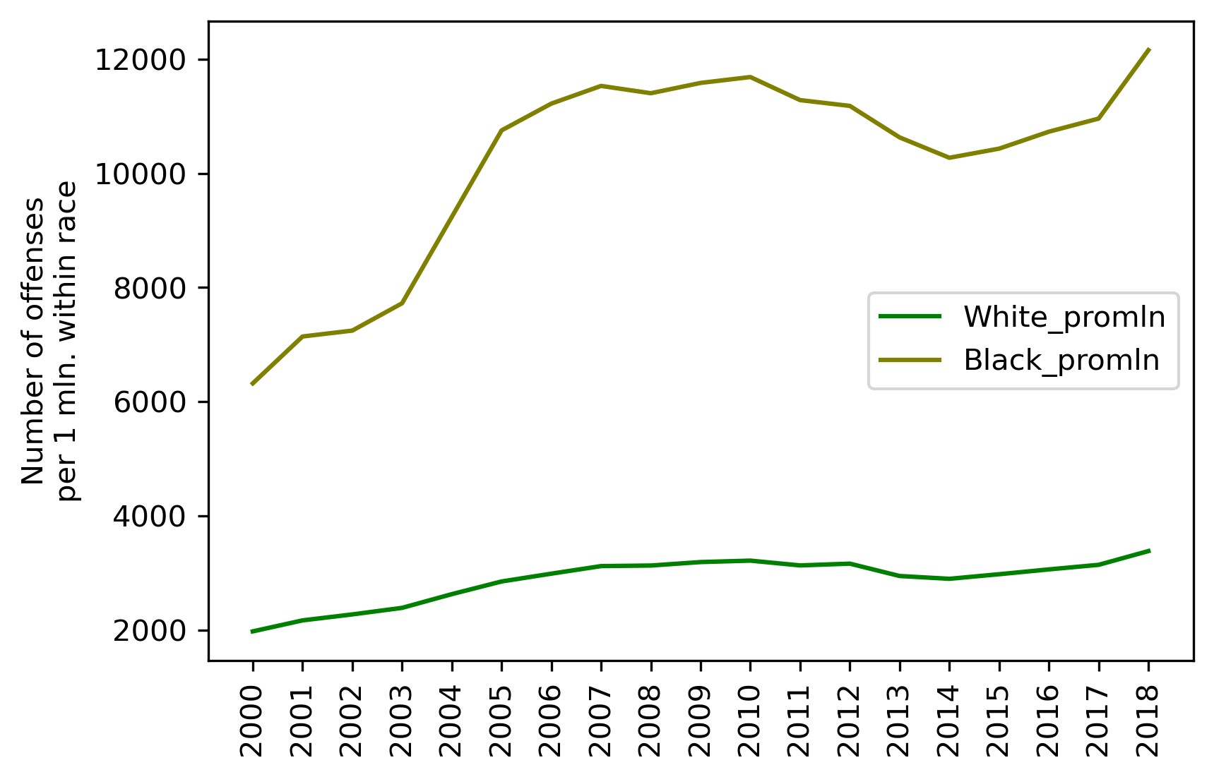
We can see that, though the scale (Y-axis) is much lower, the shape of the curves is almost identical to the All Offenses ones we saw previously.
The criminality vs. lethal force victims curves for both races:
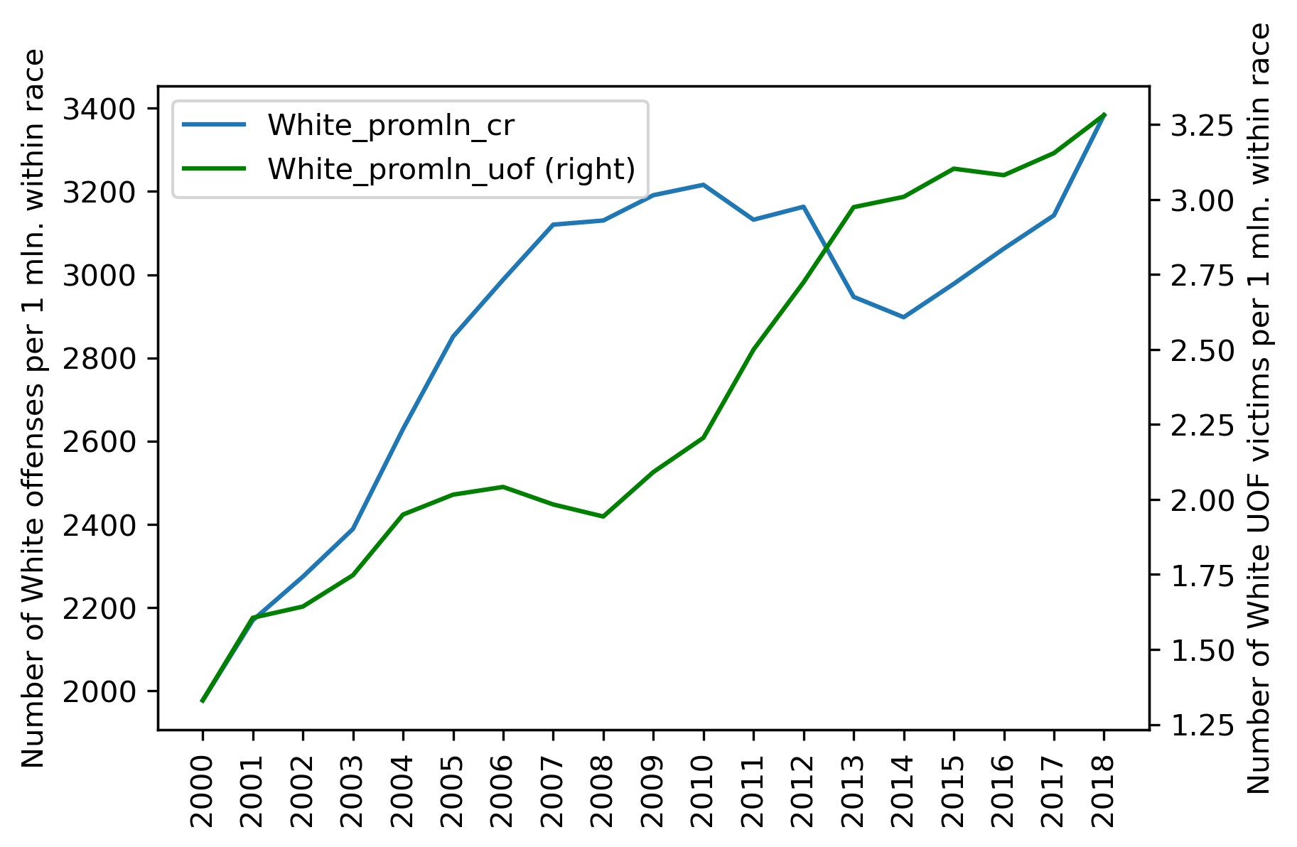

And the correlation matrix:
| White_promln_cr | White_promln_uof | Black_promln_cr | Black_promln_uof | |
|---|---|---|---|---|
| White_promln_cr | 1.000000 | 0.684757 | 0.986622 | 0.729674 |
| White_promln_uof | 0.684757 | 1.000000 | 0.614132 | 0.795486 |
| Black_promln_cr | 0.986622 | 0.614132 | 1.000000 | 0.680893 |
| Black_promln_uof | 0.729674 | 0.795486 | 0.680893 | 1.000000 |
The correlation between criminality and lethal force fatalities is worse this time (0.68 against 0.88 and 0.72 for All Offenses). But the silver lining here is the fact that the correlation coefficients for Whites and Blacks are almost equal, which gives reason to say there is some constant correlation between crime and police shootings / victims (regardless of race).
Now for our 'DIY' index — the ratio of lethal force deaths to the number of crimes (both per capita):
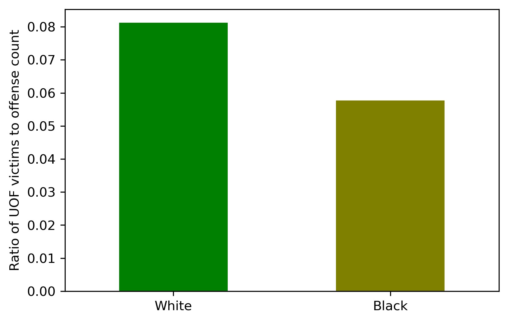
The difference here is even more apparent. The inference is the same: White criminals are more likely to get killed by the police than Black criminals.
The summary is that all our prior conclusions hold true.
Well, down to geography lessons now! :)
Source Data
To investigate criminality in individual states, I used different source endpoints in the FBI database:
- State level UCR Estimated Crime Data Endpoint — without race classification (the resulting CSV can be downloaded from here)
- State level Arrest Demographic Count By Offense Endpoint — with race classification (the resulting CSV can be downloaded from here)
Unfortunately, I didn't manage to get complete data on committed offenses with the offense state, year and offender race, much as I tried. The returned results had large gaps, for example, some states were totally omitted. But the alternative data on arrests is quite sufficient for our humble research.
The first dataset contains crime counts for all the 51 states from 1991 to 2018, for the following offense categories:
- violent crime (murder, rape, robbery and aggravated assault)
- homicide (all types, including negligent / justifiable)
- rape legacy (using outdated metrics — before 2013)
- rape revised (using updated metrics — from 2013 on)
- robbery
- aggravated assault
- property crime
- burglary
- larceny
- motor vehicle theft
- arson
For our purposes, we'll be using the 'violent crime' category, in keeping with the rest of the research.
The second dataset features the number of arrests for the 51 states from 2000 to 2018, with details on the arrested persons' race (refer to the previous part for the race categories). Since the arrest dataset uses a different offense classification and doesn't provide the combined 'violent crime' category, the requests and retrieved results are for the four constituent offenses — murder / non-negligent manslaughter, robbery, rape, and aggravated assault.
Crime Distribution (No Racial Factor)
First, we'll look at the distribution of violent crimes across the states regardless of the offenders' race:
import pandas as pd, numpy as np

CRIME_STATES_FILE = ROOT_FOLDER + '\\crimes_by_state.csv'
df_crime_states = pd.read_csv(CRIME_STATES_FILE, sep=';', header=0,
                         usecols=['year', 'state_abbr', 'population', 'violent_crime'])
The resulting dataset:
| year | state_abbr | population | violent_crime | |
|---|---|---|---|---|
| 0 | 2016 | AL | 4860545 | 25878 |
| 1 | 1996 | AL | 4273000 | 24159 |
| 2 | 1997 | AL | 4319000 | 24379 |
| 3 | 1998 | AL | 4352000 | 22286 |
| 4 | 1999 | AL | 4369862 | 21421 |
| ... | ... | ... | ... | ... |
| 1423 | 2000 | DC | 572059 | 8626 |
| 1424 | 2001 | DC | 573822 | 9195 |
| 1425 | 2002 | DC | 569157 | 9322 |
| 1426 | 2003 | DC | 557620 | 9061 |
| 1427 | 2016 | DC | 684336 | 8236 |
1428 rows × 4 columns
Adding the full state names (the list of states we already used in our research — CSV) and optimizing / sorting the data:
df_crime_states = df_crime_states.merge(df_state_names, on='state_abbr')
df_crime_states.dropna(inplace=True)
df_crime_states.sort_values(by=['year', 'state_abbr'], inplace=True)
Since the dataset already has population values, let's calculate the number of crimes per million people:
df_crime_states['crime_promln'] = df_crime_states['violent_crime'] * 1e6 /
                                             df_crime_states['population']
Finally, we'll turn the data into a table spanning the 2000 — 2018 period transposing the state names and dropping the redundant columns:
df_crime_states_agg = df_crime_states.groupby(['state_name',
                                 'year'])['violent_crime'].sum().unstack(level=1).T
df_crime_states_agg.fillna(0, inplace=True)
df_crime_states_agg = df_crime_states_agg.astype('uint32').loc[2000:2018, :]
The resulting table contains 19 rows (year observations from 2000 through 2018) and 51 columns (by the number of states).
Let's display the top 10 states for the average number of crimes:
df_crime_states_agg_top10 = df_crime_states_agg.describe().T.nlargest(10, 'mean').\
                                                                                                         astype('uint32')
| count | mean | std | min | 25% | 50% | 75% | max | |
|---|---|---|---|---|---|---|---|---|
| state_name | ||||||||
| California | 19 | 181514 | 19425 | 153763 | 165508 | 178597 | 193022 | 212867 |
| Texas | 19 | 117614 | 6522 | 104734 | 113212 | 121091 | 122084 | 126018 |
| Florida | 19 | 110104 | 18542 | 81980 | 92809 | 113541 | 127488 | 131878 |
| New York | 19 | 81618 | 9548 | 68495 | 75549 | 77563 | 85376 | 105111 |
| Illinois | 19 | 62866 | 10445 | 47775 | 54039 | 64185 | 69937 | 81196 |
| Michigan | 19 | 49273 | 5029 | 41712 | 44900 | 49737 | 54035 | 56981 |
| Pennsylvania | 19 | 46941 | 5066 | 39192 | 41607 | 48188 | 51021 | 55028 |
| Tennessee | 19 | 41951 | 2432 | 38063 | 40321 | 41562 | 43358 | 46482 |
| Georgia | 19 | 40228 | 3327 | 34355 | 38283 | 39435 | 41495 | 47353 |
| North Carolina | 19 | 37936 | 3193 | 32718 | 34706 | 38243 | 40258 | 43125 |
We'll also make it more graphic with a box plot:
df_crime_states_top10 = df_crime_states_agg.loc[:, df_crime_states_agg_top10.index]
plt = df_crime_states_top10.plot.box(figsize=(12, 10))
plt.set_ylabel('Violent crime count (2000 - 2018)')

The 'Hollywood' state easily and notoriously beats the rest 9. The 'prizewinners' are California, Texas and Florida, all three in the South, the regular settings for most Hollywood criminal blockbusters.
You can also see that criminality has changed considerably over the observed period in some states (California, Florida and Illinois), whereas in others (like Georgia) it has remained almost constant.
I tend to think the crime rates are in some way connected with population :) Let's see the top 10 states by population in 2018:
df_crime_states_2018 = df_crime_states.loc[df_crime_states['year'] == 2018]
plt = df_crime_states_2018.nlargest(10, 'population').\
                                       sort_values(by='population').plot.barh(x='state_name',
                                       y='population', legend=False, figsize=(10,5))
plt.set_xlabel('2018 Population')
plt.set_ylabel('')

Same old mugs here :) Let's check the correlation between crimes and population:
df_corr = df_crime_states[df_crime_states['year']>=2000].groupby(['state_name']).mean()
df_corr = df_corr.loc[:, ['population', 'violent_crime']]
df_corr.corr(method='pearson').at['population', 'violent_crime']
The calculated Pearson correlation coefficient is 0.98. Q.E.D.
But the per capita crime counts give a staringly different picture:
plt = df_crime_states_2018.nlargest(10, 'crime_promln').\
                                sort_values(by='crime_promln').plot.barh(x='state_name',
                                y='crime_promln', legend=False, figsize=(10,5))
plt.set_xlabel('Number of violent crimes per 1 mln. population (2018)')
plt.set_ylabel('')
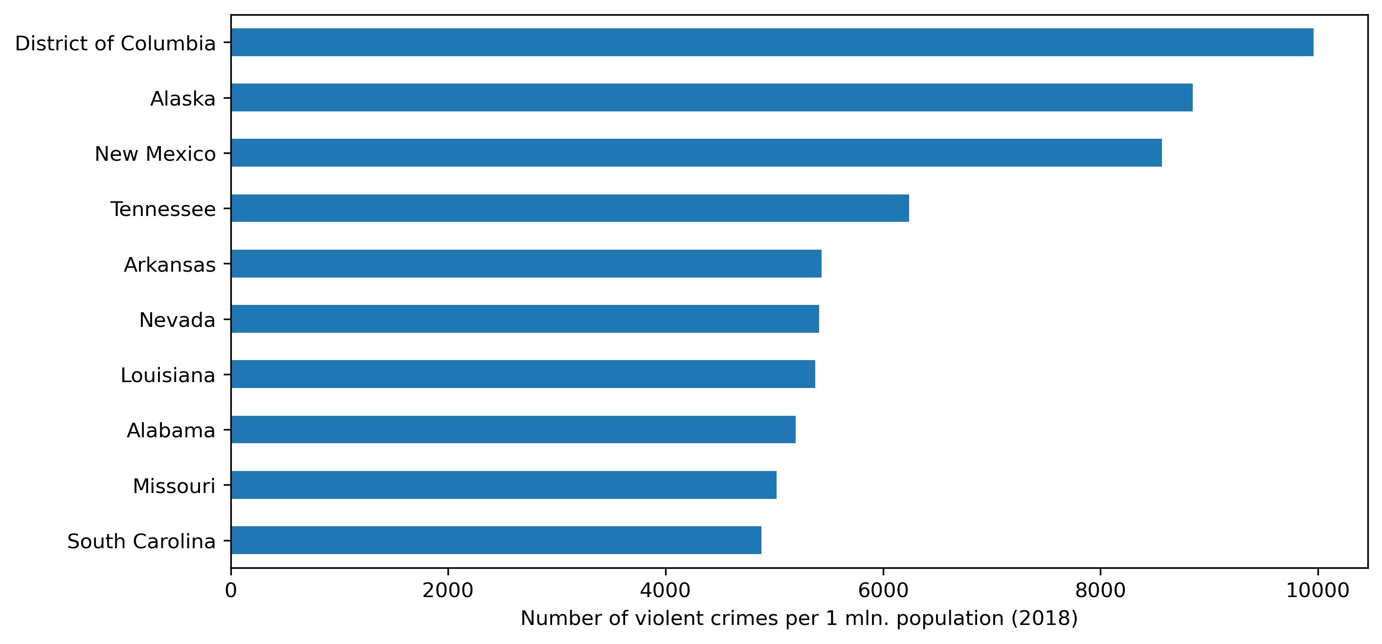
There's a pretty kettle of fish! The leaders by per capita crimes are the least populated states: District Columbia (with the US capital) and Alaska (both home to some 700+ thousand people as of 2018), as well as one medium-populated state — New Mexico, with 2 mln. people. Only one state from our previous toplist is featured here — Tennessee, which gives this state a less-than-desirable reputation.
We will then display these results on the US map. To do this, we need the folium library:
import folium
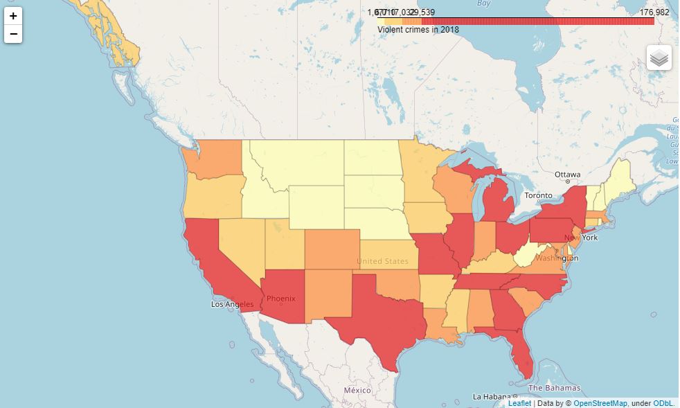
First, the 2018 absolute crime counts:
FOLIUM_URL = 'https://raw.githubusercontent.com/python-visualization/folium/master/examples/data'
FOLIUM_US_MAP = f'{FOLIUM_URL}/us-states.json'

m = folium.Map(location=[48, -102], zoom_start=3)

folium.Choropleth(
    geo_data=FOLIUM_US_MAP,
    name='choropleth',
    data=df_crime_states_2018,
    columns=['state_abbr', 'violent_crime'],
    key_on='feature.id',
    fill_color='YlOrRd',
    fill_opacity=0.7,
    line_opacity=0.2,
    legend_name='Violent crimes in 2018',
    bins=df_crime_states_2018['violent_crime'].quantile(
                                            list(np.linspace(0.0, 1.0, 5))).to_list(),
    reset=True
).add_to(m)

folium.LayerControl().add_to(m)

m
The same in per capita values (per 1 million):
m = folium.Map(location=[48, -102], zoom_start=3)

folium.Choropleth(
    geo_data=FOLIUM_US_MAP,
    name='choropleth',
    data=df_crime_states_2018,
    columns=['state_abbr', 'crime_promln'],
    key_on='feature.id',
    fill_color='YlOrRd',
    fill_opacity=0.7,
    line_opacity=0.2,
    legend_name='Violent crimes in 2018 (per 1 mln. population)',
    bins=df_crime_states_2018['crime_promln'].quantile(
                                             list(np.linspace(0.0, 1.0, 5))).to_list(),
    reset=True
).add_to(m)

folium.LayerControl().add_to(m)

m
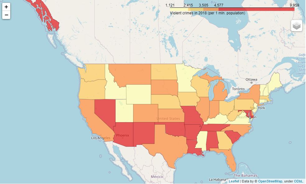
In the first case, as we can see, crimes are more or less evenly distributed in the North to South direction. In the second case, it's mostly the Southern states plus DC and Alaska that make the trend.
Lethal Force Fatalities Across States (No Racial Factor)
We are now going to look at lethal force used in individual states across the country.
To prepare the dataset, we'll complement the UOF (Use Of Force) data we used previously by the full state names, group the cases by states, and constrain the observations to years 2000 through 2018:
df_fenc_agg_states = df_fenc.merge(df_state_names, how='inner',
                                         left_on='State', right_on='state_abbr')
df_fenc_agg_states.fillna(0, inplace=True)
df_fenc_agg_states = df_fenc_agg_states.rename(columns={'state_name_x': 'State Name'})
df_fenc_agg_states = df_fenc_agg_states.loc[:, ['Year', 'Race', 'State',
                                                'State Name', 'Cause', 'UOF']]

df_fenc_agg_states = df_fenc_agg_states.\
                                groupby(['Year', 'State Name', 'State'])['UOF'].\
                                count().unstack(level=0)
df_fenc_agg_states.fillna(0, inplace=True)
df_fenc_agg_states = df_fenc_agg_states.astype('uint16').loc[:, :2018]
df_fenc_agg_states = df_fenc_agg_states.reset_index()
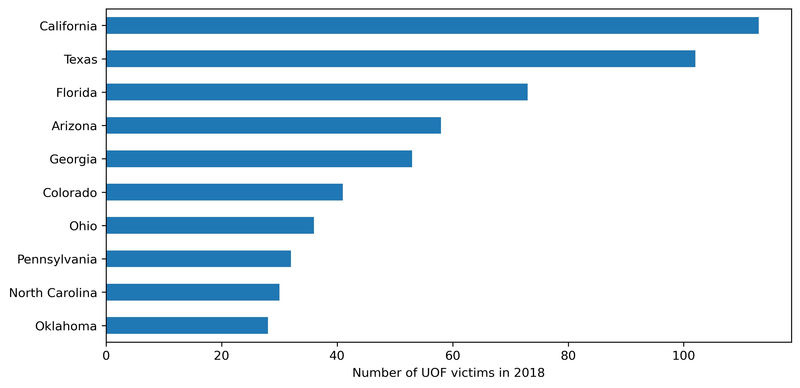
Top 10 states for police victims in 2018:
df_fenc_agg_states_2018 = df_fenc_agg_states.loc[:, ['State Name', 2018]]
plt = df_fenc_agg_states_2018.nlargest(10, 2018).sort_values(2018).plot.barh(
                                   x='State Name', y=2018, legend=False, figsize=(10,5))
plt.set_xlabel('Number of UOF victims in 2018')
plt.set_ylabel('')
Let's also review the data for the entire period as a box plot:
fenc_top10 = df_fenc_agg_states.loc[df_fenc_agg_states['State Name'].\
            isin(df_fenc_agg_states_2018.nlargest(10, 2018)['State Name'])]
fenc_top10 = fenc_top10.T
fenc_top10.columns = fenc_top10.loc['State Name', :]
fenc_top10 = fenc_top10.reset_index().loc[2:, :].set_index('Year')
df_sorted = fenc_top10.mean().sort_values(ascending=False)
fenc_top10 = fenc_top10.loc[:, df_sorted.index]

plt = fenc_top10.plot.box(figsize=(12, 6))
plt.set_ylabel('Number of UOF victims (2000 - 2018)')
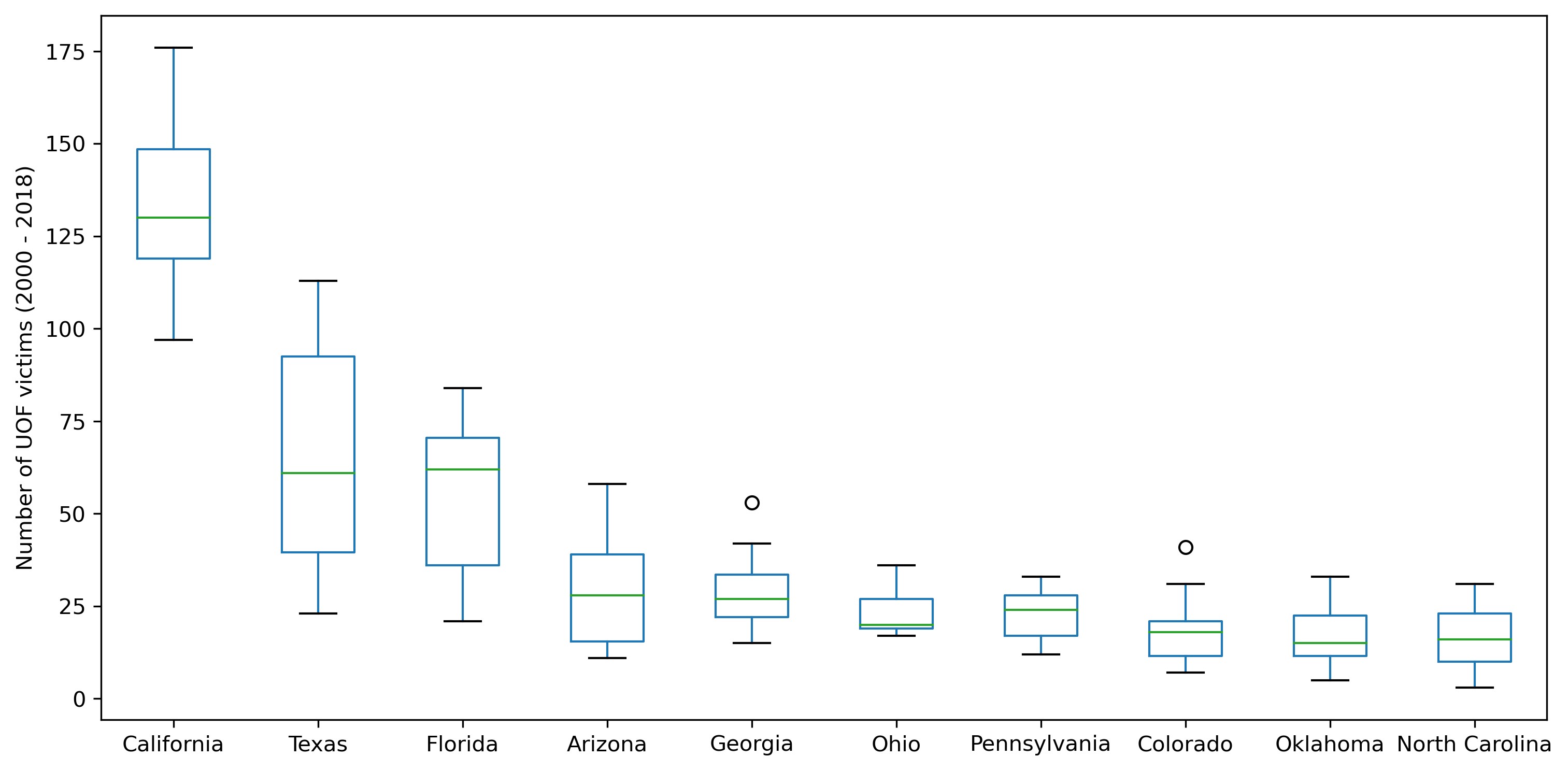
Yep! The same 'unholy trio' of California, Texas and Florida, with their other two Southern sidekicks — Arizona and Georgia. The leaders again show large scatter indicative of year-to-year changes.
Connection Between Lethal Force Fatalities and Crimes
As in the previous part of this research, we are investigating the possible connection between criminality and deaths at the hands of law enforcement. We'll start without the racial factor, to see if such a connection exists in principle and how it varies from state to state.
At first, we must merge the UOF and (violent) crime datasets, setting the observation period to 2000 — 2018:
# add full state names
df_fenc_crime_states = df_fenc.merge(df_state_names, how='inner',
                                   left_on='State', right_on='state_abbr')
# rename some columns
df_fenc_crime_states = df_fenc_crime_states.rename(columns={'Year': 'year',
                                   'state_name_x': 'state_name'})
# truncate period to 2000-2018
df_fenc_crime_states = df_fenc_crime_states[df_fenc_crime_states['year'].between(2000,
                                                                            2018)]
# group by year and state
df_fenc_crime_states = df_fenc_crime_states.groupby(['year', 'state_name'])['UOF'].\
                                  count().reset_index()
# join with crime data
df_fenc_crime_states = df_fenc_crime_states.merge(df_crime_states[df_crime_states['year'].\
                             between(2000, 2018)], how='outer', on=['year', 'state_name'])
# set missing data to zero
df_fenc_crime_states.fillna({'UOF': 0}, inplace=True)
# unify data types
df_fenc_crime_states = df_fenc_crime_states.astype({'year': 'uint16', 'UOF': 'uint16',
                                  'population': 'uint32', 'violent_crime': 'uint32'})
# sort data
df_fenc_crime_states = df_fenc_crime_states.sort_values(by=['year', 'state_name'])
Resulting dataset
| year | state_name | UOF | state_abbr | population | violent_crime | crime_promln | |
|---|---|---|---|---|---|---|---|
| 0 | 2000 | Alabama | 7 | AL | 4447100 | 21620 | 4861.595197 |
| 1 | 2000 | Alaska | 2 | AK | 626932 | 3554 | 5668.876369 |
| 2 | 2000 | Arizona | 11 | AZ | 5130632 | 27281 | 5317.278651 |
| 3 | 2000 | Arkansas | 4 | AR | 2673400 | 11904 | 4452.756789 |
| 4 | 2000 | California | 97 | CA | 33871648 | 210531 | 6215.552311 |
| ... | ... | ... | ... | ... | ... | ... | ... |
| 907 | 2018 | Virginia | 18 | VA | 8517685 | 17032 | 1999.604353 |
| 908 | 2018 | Washington | 24 | WA | 7535591 | 23472 | 3114.818732 |
| 909 | 2018 | West Virginia | 7 | WV | 1805832 | 5236 | 2899.494527 |
| 910 | 2018 | Wisconsin | 10 | WI | 5813568 | 17176 | 2954.467893 |
| 911 | 2018 | Wyoming | 4 | WY | 577737 | 1226 | 2122.072846 |
As you will remember, the UOF column contains the number of deaths from encounters with law enforcement officers (who I sometimes call here just 'the police', but who include, of course, other agencies such as the FBI) where lethal force was used intentionally.
We will also make a separate dataset with year-average values:
df_fenc_crime_states_agg = df_fenc_crime_states.groupby(['state_name']).\
                            mean().loc[:, ['UOF', 'violent_crime']]
Now let's look at the year averages for crimes and lethal force fatalities for all the 51 states on one plot:
plt = df_fenc_crime_states_agg['violent_crime'].plot.bar(legend=True, figsize=(15,5))
plt.set_ylabel('Number of violent crimes (year average)')
plt2 = df_fenc_crime_states_agg['UOF'].plot(secondary_y=True, style='g', legend=True)
plt2.set_ylabel('Number of UOF victims (year average)', rotation=90)
plt2.set_xlabel('')
plt.set_xlabel('')
plt.set_xticklabels(df_fenc_crime_states_agg.index, rotation='vertical')
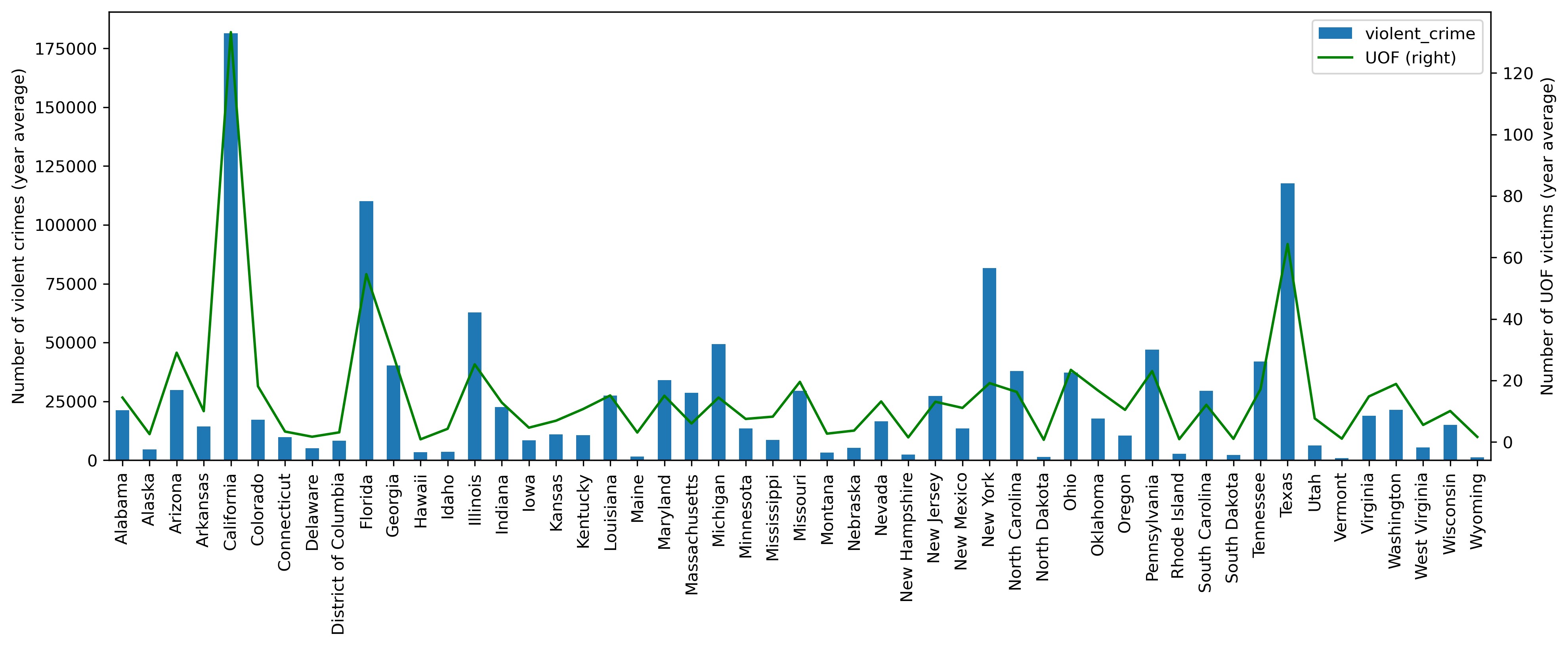
Looking closely at this combined chart, one can see the following:
- the connection between crime and use of force is plainly trackable: the green UOF curve tends to repeat the shape of the crime bars
- the more criminal states (such as Florida, Illinois, Michigan, New York and Texas) evince proportionately less use of force compared to the less criminal states
Let's also make a scatterplot:
plt = df_fenc_crime_states_agg.plot.scatter(x='violent_crime', y='UOF')
plt.set_xlabel('Number of violent crimes (year average)')
plt.set_ylabel('Number of UOF victims (year average)')

Here it becomes conspicuous that the ratio between crime and use of lethal force is affected by the crime rate. Speaking crudely, in states with the number of violent crimes below 75k the number of police victims grows more slowly; whereas in the states with the crime count above 75k this growth is quite steep. This latter group includes, as we can see, only four states. Let's look them 'in the face':
df_fenc_crime_states_agg[df_fenc_crime_states_agg['violent_crime'] > 75000]
| UOF | violent_crime | |
|---|---|---|
| state_name | ||
| California | 133.263158 | 181514.578947 |
| Florida | 54.578947 | 110104.315789 |
| New York | 19.157895 | 81618.052632 |
| Texas | 64.368421 | 117614.631579 |
Will you be surprised? We've got the same 'four horsemen of the Apocalypse': California, Florida, Texas and New York.
Correspondingly, let's calculate the correlation coefficients between our data for three cases:
- states with the year average crime count up to 75,000
- states with the year average crime count above 75,000
- all the states
For the first case:
df_fenc_crime_states_agg[df_fenc_crime_states_agg['violent_crime'] <= \
                  75000].corr(method='pearson').at['UOF', 'violent_crime']
— we obtain 0.839 as the correlation coefficient. This is a statistically valid value, although it doesn't reach 0.9 due to scatter across the 47 states.
For the first case:
df_fenc_crime_states_agg[df_fenc_crime_states_agg['violent_crime'] > \
                  75000].corr(method='pearson').at['UOF', 'violent_crime']
— we get 0.999 — an ideal correlation!
For the last case (all states):
df_fenc_crime_states_agg.corr(method='pearson').at['UOF', 'violent_crime']
— the correlation is estimated at 0.935. This overall correlation may be considered very good.
Let's now look at the geographical distribution of our 'offender shootdown' index (the term is coined here for brevity). As before, we divide the number of lethal force fatalities by the number of crimes:
df_fenc_crime_states_agg['uof_by_crime'] = df_fenc_crime_states_agg['UOF'] /
                                  df_fenc_crime_states_agg['violent_crime']
plt = df_fenc_crime_states_agg.loc[:, 'uof_by_crime'].sort_values(ascending=False).\
                                  plot.bar(figsize=(15,5))
plt.set_xlabel('')
plt.set_ylabel('Ratio of UOF victims to number of violent crimes')
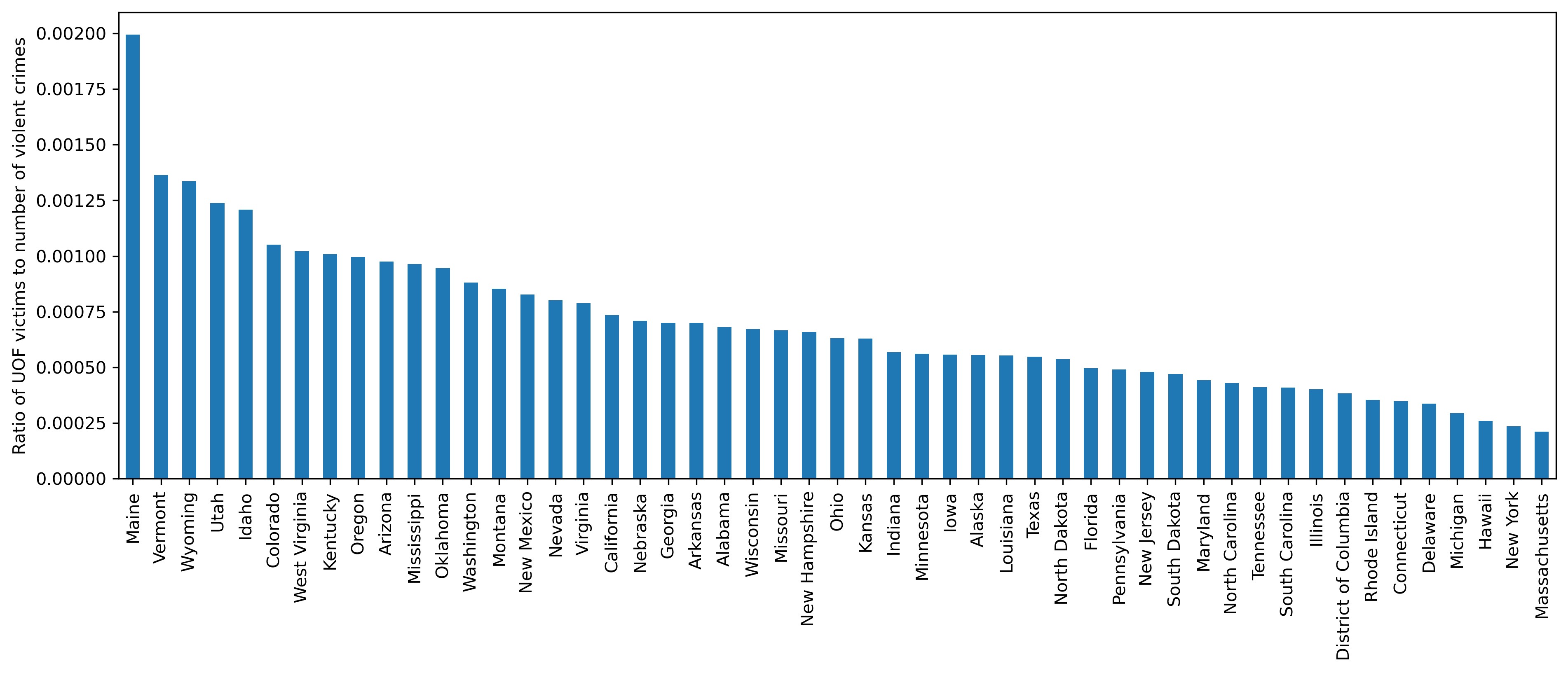
It is interesting to observe that our erstwhile leaders have shifted toward the center or even the rightmost end of the chart, which must mean that the most criminal states don't have the most 'bloodthirsty' police (towards real or potential offenders).
Intermediate conclusions:
- The number of violent crimes is directly proportionate to population (good call, Captain Obvious!)
- The most populated states (California, Florida, Texas and New York) are also the most criminal, in absolute values.
- In per capita values, Southern states are more criminal than Northern states, with the exception of Alaska and District Columbia.
- Lethal force deaths are correlated to criminality with an average coefficient of 0.93 across all the states. This correlation reaches almost unity (strictly linear) for the most criminal states and only 0.84 for the rest.
Racial Factor in Criminality and Lethal Force Fatalities Across States
Proving that crime rates do affect police victim rates, let's add the racial factor and see what it affects. As I explained above, we'll be using the arrest data for this purpose as being the most complete and covering the main offenses for all the states. There is, of course, no such state or country where one could equate the number of committed crimes to the number of arrests; yet these parameters are closely related. As such, we can do very well with arrest data for our statistical analysis. And, as we already agreed, only violent offenses (murder, rape, robbery, aggravated assault) will be taken into account.
Let's load the source data from the CSV file and routinely add the full state names:
ARRESTS_FILE = ROOT_FOLDER + '\\arrests_by_state_race.csv'
# arrests of Blacks and Whites only
df_arrests = pd.read_csv(ARRESTS_FILE, sep=';', header=0,
                      usecols=['data_year', 'state', 'white', 'black'])
# sum the four offenses and group by states
df_arrests = df_arrests.groupby(['data_year', 'state']).sum().reset_index()
# add state names
df_arrests = df_arrests.merge(df_state_names, left_on='state', right_on='state_abbr')
# rename / remove columns
df_arrests = df_arrests.rename(columns={'data_year': 'year'}).drop(columns='state_abbr')
# peek at the result
df_arrests.head()
| year | state | black | white | state_name | |
|---|---|---|---|---|---|
| 0 | 2000 | AK | 140 | 613 | Alaska |
| 1 | 2001 | AK | 139 | 718 | Alaska |
| 2 | 2002 | AK | 143 | 677 | Alaska |
| 3 | 2003 | AK | 173 | 801 | Alaska |
| 4 | 2004 | AK | 163 | 765 | Alaska |
We'll also create a dataframe with year average values:
df_arrests_agg = df_arrests.groupby(['state_name']).mean().drop(columns='year')
Arrests of Whites and Blacks in 51 states (year average counts)
| black | white | |
|---|---|---|
| state_name | ||
| Alabama | 2805.842105 | 1757.315789 |
| Alaska | 221.894737 | 844.157895 |
| Arizona | 1378.368421 | 7007.157895 |
| Arkansas | 2387.894737 | 2303.789474 |
| California | 26668.368421 | 87252.315789 |
| Colorado | 1268.210526 | 5157.368421 |
| Connecticut | 2097.631579 | 2981.210526 |
| Delaware | 1356.894737 | 1048.578947 |
| District of Columbia | 111.111111 | 4.944444 |
| Florida | 12.000000 | 7.000000 |
| Georgia | 8262.842105 | 3502.894737 |
| Hawaii | 81.052632 | 368.736842 |
| Idaho | 44.000000 | 1362.263158 |
| Illinois | 5699.842105 | 1841.894737 |
| Indiana | 3553.368421 | 5192.263158 |
| Iowa | 1104.421053 | 3039.473684 |
| Kansas | 522.315789 | 1501.315789 |
| Kentucky | 1476.894737 | 1906.052632 |
| Louisiana | 5928.789474 | 3414.263158 |
| Maine | 63.736842 | 699.526316 |
| Maryland | 7189.105263 | 4010.684211 |
| Massachusetts | 3407.157895 | 7319.684211 |
| Michigan | 7628.157895 | 6304.157895 |
| Minnesota | 2231.210526 | 2645.736842 |
| Mississippi | 1462.210526 | 474.368421 |
| Missouri | 5777.473684 | 5703.368421 |
| Montana | 27.684211 | 673.684211 |
| Nebraska | 591.421053 | 1058.526316 |
| Nevada | 1956.421053 | 3817.210526 |
| New Hampshire | 68.368421 | 640.789474 |
| New Jersey | 6424.157895 | 6043.789474 |
| New Mexico | 234.421053 | 2809.368421 |
| New York | 8394.526316 | 8734.947368 |
| North Carolina | 10527.947368 | 7412.947368 |
| North Dakota | 61.263158 | 277.052632 |
| Ohio | 4063.947368 | 4071.368421 |
| Oklahoma | 1625.105263 | 3353.000000 |
| Oregon | 445.105263 | 3373.368421 |
| Pennsylvania | 11974.157895 | 11039.473684 |
| Rhode Island | 275.684211 | 699.210526 |
| South Carolina | 5578.526316 | 3615.421053 |
| South Dakota | 67.105263 | 349.368421 |
| Tennessee | 6799.894737 | 8462.526316 |
| Texas | 10547.631579 | 22062.684211 |
| Utah | 167.105263 | 1748.894737 |
| Vermont | 43.526316 | 439.210526 |
| Virginia | 4100.421053 | 3060.263158 |
| Washington | 1688.947368 | 6012.105263 |
| West Virginia | 271.263158 | 1528.315789 |
| Wisconsin | 3440.055556 | 4107.722222 |
| Wyoming | 27.263158 | 506.947368 |
Looking at this table, one can't overlook some oddities. In some states the arrest counts reach hundreds and thousands, while in others — only dozens or fewer. That's the case with Florida, one of the most populated states: it counts only 19 arrests per year (12 Blacks and 7 Whites). Surely, some data is missing here; let's check:
df_arrests[df_arrests['state'] == 'FL']
And indeed we see that data for Florida is available only for 2017. Well, we'll have to put up with this, I suppose. All the other states have complete data. But the ten / hundred-fold difference should be accounted for by population. Let's add population-by-race data and have a look.
The population data was taken from the US Census Bureau website (which is for some reason not accessible in Russia). You can download the prepared CSV file with 2010 — 2019 data from here.
Unfortunately, no state population data exist for prior periods (2000 — 2009). We have therefore to narrow down our observation period to 9 years (from 2010 through 2018) for this part of the research.
POP_STATES_FILES = ROOT_FOLDER + '\\us_pop_states_race_2010-2019.csv'
df_pop_states = pd.read_csv(POP_STATES_FILES, sep=';', header=0)
# the source CSV has a specific format, so some trickery is required :)
df_pop_states = df_pop_states.melt('state_name', var_name='r_year', value_name='pop')
df_pop_states['race'] = df_pop_states['r_year'].str[0]
df_pop_states['year'] = df_pop_states['r_year'].str[2:].astype('uint16')
df_pop_states.drop(columns='r_year', inplace=True)
df_pop_states = df_pop_states[df_pop_states['year'].between(2000, 2018)]
df_pop_states = df_pop_states.groupby(['state_name', 'year', 'race']).sum().\
                                         unstack().reset_index()
df_pop_states.columns = ['state_name', 'year', 'black_pop', 'white_pop']
White and Black population across states
| year | black_pop | white_pop | |
|---|---|---|---|
| state_name | |||
| Alabama | 2010 | 5044936 | 13462236 |
| Alabama | 2011 | 5067912 | 13477008 |
| Alabama | 2012 | 5102512 | 13484256 |
| Alabama | 2013 | 5137360 | 13488812 |
| Alabama | 2014 | 5162316 | 13493432 |
| ... | ... | ... | ... |
| Wyoming | 2014 | 31392 | 2167008 |
| Wyoming | 2015 | 29568 | 2177740 |
| Wyoming | 2016 | 29304 | 2170700 |
| Wyoming | 2017 | 29444 | 2148128 |
| Wyoming | 2018 | 29604 | 2139896 |
Merging this data with the arrests dataset, we can calculate the per-million arrest counts:
df_arrests_2010_2018 = df_arrests.merge(df_pop_states, how='inner',
                                             on=['year', 'state_name'])
df_arrests_2010_2018['white_arrests_promln'] = df_arrests_2010_2018['white'] * 1e6 /
                                             df_arrests_2010_2018['white_pop']
df_arrests_2010_2018['black_arrests_promln'] = df_arrests_2010_2018['black'] * 1e6 /
                                             df_arrests_2010_2018['black_pop']
And again let's calculate the year averages:
df_arrests_2010_2018_agg = df_arrests_2010_2018.groupby(
         ['state_name', 'state']).mean().drop(columns='year').reset_index()
df_arrests_2010_2018_agg = df_arrests_2010_2018_agg.set_index('state_name')
Combined arrest dataset with absolute and per-million counts
| state | black | white | black_pop | white_pop | white_arrests_promln | black_arrests_promln | |
|---|---|---|---|---|---|---|---|
| state_name | |||||||
| Alabama | AL | 1682.000000 | 1342.000000 | 5.152399e+06 | 1.349158e+07 | 99.424741 | 324.055203 |
| Alaska | AK | 255.000000 | 870.555556 | 1.069489e+05 | 1.957445e+06 | 445.199704 | 2390.243876 |
| Arizona | AZ | 1635.555556 | 6852.000000 | 1.279172e+06 | 2.260403e+07 | 302.923002 | 1267.000192 |
| Arkansas | AR | 1960.666667 | 2466.000000 | 1.855574e+06 | 9.465137e+06 | 260.459917 | 1055.854934 |
| California | CA | 24381.666667 | 79477.000000 | 1.007921e+07 | 1.128020e+08 | 704.731408 | 2419.234376 |
| Colorado | CO | 1377.222222 | 5171.555556 | 9.508173e+05 | 1.882940e+07 | 274.209456 | 1439.257054 |
| Connecticut | CT | 1823.777778 | 2295.333333 | 1.643690e+06 | 1.165681e+07 | 196.712775 | 1114.811569 |
| Delaware | DE | 1318.000000 | 914.111111 | 8.354622e+05 | 2.635794e+06 | 347.374980 | 1582.395733 |
| District of Columbia | DC | 139.222222 | 4.777778 | 1.288488e+06 | 1.154416e+06 | 4.112547 | 108.101938 |
| Florida | FL | 12.000000 | 7.000000 | 1.415383e+07 | 6.498292e+07 | 0.107721 | 0.847827 |
| Georgia | GA | 8137.222222 | 4271.444444 | 1.279378e+07 | 2.500293e+07 | 170.939250 | 639.869143 |
| Hawaii | HI | 81.333333 | 383.777778 | 1.124298e+05 | 1.453712e+06 | 264.353469 | 725.477589 |
| Idaho | ID | 51.888889 | 1373.777778 | 5.288222e+04 | 6.154316e+06 | 223.151878 | 978.205026 |
| Illinois | IL | 4216.000000 | 1284.222222 | 7.554687e+06 | 3.980927e+07 | 32.199075 | 557.493894 |
| Indiana | IN | 2924.444444 | 5186.111111 | 2.522917e+06 | 2.267508e+07 | 228.699515 | 1155.168768 |
| Iowa | IA | 1181.000000 | 2999.222222 | 4.305640e+05 | 1.141794e+07 | 262.666753 | 2760.038539 |
| Kansas | KS | 539.555556 | 1512.111111 | 7.116182e+05 | 1.006714e+07 | 150.232160 | 758.851182 |
| Kentucky | KY | 1443.888889 | 2173.666667 | 1.442174e+06 | 1.558094e+07 | 139.526970 | 1001.433470 |
| Louisiana | LA | 5917.000000 | 3255.333333 | 6.021228e+06 | 1.174245e+07 | 277.277874 | 981.334817 |
| Maine | ME | 78.000000 | 678.000000 | 7.667733e+04 | 5.059062e+06 | 134.024032 | 1019.061684 |
| Maryland | MD | 6460.444444 | 3325.444444 | 7.229037e+06 | 1.426036e+07 | 233.317775 | 893.942720 |
| Massachusetts | MA | 3349.555556 | 6895.111111 | 2.249232e+06 | 2.226671e+07 | 309.745910 | 1505.096888 |
| Michigan | MI | 6302.444444 | 5647.444444 | 5.645176e+06 | 3.170670e+07 | 178.111684 | 1116.364030 |
| Minnesota | MN | 2570.000000 | 2686.777778 | 1.311818e+06 | 1.867259e+07 | 143.902882 | 1986.464052 |
| Mississippi | MS | 1251.000000 | 418.777778 | 4.478208e+06 | 7.122651e+06 | 58.753686 | 279.574565 |
| Missouri | MO | 4588.333333 | 5146.111111 | 2.854060e+06 | 2.023871e+07 | 254.292323 | 1608.303611 |
| Montana | MT | 34.222222 | 788.333333 | 2.210444e+04 | 3.660813e+06 | 214.944902 | 1525.795754 |
| Nebraska | NE | 618.888889 | 1154.888889 | 3.701520e+05 | 6.709768e+06 | 172.269972 | 1687.725359 |
| Nevada | NV | 2450.000000 | 4480.333333 | 1.052192e+06 | 8.647157e+06 | 517.401564 | 2316.374085 |
| New Hampshire | NH | 89.777778 | 784.777778 | 7.873600e+04 | 5.012056e+06 | 156.580888 | 1141.127571 |
| New Jersey | NJ | 5429.555556 | 4971.888889 | 5.241910e+06 | 2.595141e+07 | 191.427955 | 1037.217679 |
| New Mexico | NM | 260.111111 | 3136.000000 | 2.053876e+05 | 6.905377e+06 | 454.129135 | 1268.115549 |
| New York | NY | 6035.777778 | 6600.222222 | 1.373077e+07 | 5.534157e+07 | 119.253616 | 439.581451 |
| North Carolina | NC | 9549.000000 | 6759.333333 | 8.804027e+06 | 2.844145e+07 | 238.320077 | 1088.968561 |
| North Dakota | ND | 100.666667 | 386.222222 | 6.583289e+04 | 2.583206e+06 | 149.190455 | 1536.987272 |
| Ohio | OH | 3632.888889 | 3733.333333 | 5.879375e+06 | 3.844592e+07 | 97.107129 | 617.699379 |
| Oklahoma | OK | 1577.333333 | 3049.000000 | 1.189604e+06 | 1.160567e+07 | 262.904593 | 1326.463864 |
| Oregon | OR | 375.444444 | 3125.000000 | 3.292284e+05 | 1.402225e+07 | 222.819615 | 1148.158169 |
| Pennsylvania | PA | 11227.000000 | 10652.111111 | 5.945100e+06 | 4.232445e+07 | 251.598838 | 1893.415475 |
| Rhode Island | RI | 274.888889 | 595.000000 | 3.275551e+05 | 3.592825e+06 | 165.605635 | 837.932682 |
| South Carolina | SC | 4703.222222 | 3094.111111 | 5.365012e+06 | 1.324712e+07 | 234.287821 | 877.892998 |
| South Dakota | SD | 103.777778 | 448.333333 | 6.154533e+04 | 2.903489e+06 | 153.995184 | 1641.137012 |
| Tennessee | TN | 7603.000000 | 9068.666667 | 4.460808e+06 | 2.070126e+07 | 438.486812 | 1708.022356 |
| Texas | TX | 10821.666667 | 21122.111111 | 1.345661e+07 | 8.628389e+07 | 245.051258 | 803.917061 |
| Utah | UT | 193.222222 | 1797.333333 | 1.558876e+05 | 1.079659e+07 | 166.431266 | 1240.117890 |
| Vermont | VT | 54.222222 | 520.555556 | 3.017111e+04 | 2.376143e+06 | 219.129918 | 1785.111547 |
| Virginia | VA | 4059.555556 | 3071.222222 | 6.544598e+06 | 2.340732e+07 | 131.178648 | 620.504151 |
| Washington | WA | 1791.777778 | 5870.444444 | 1.147000e+06 | 2.289368e+07 | 256.632241 | 1566.862244 |
| West Virginia | WV | 294.111111 | 1648.666667 | 2.597649e+05 | 6.908718e+06 | 238.517207 | 1132.059057 |
| Wisconsin | WI | 3525.333333 | 4046.222222 | 1.516534e+06 | 2.018658e+07 | 200.441064 | 2325.622492 |
| Wyoming | WY | 28.777778 | 464.555556 | 2.856356e+04 | 2.151349e+06 | 216.004646 | 1005.725503 |
Let's visualize this stuff.
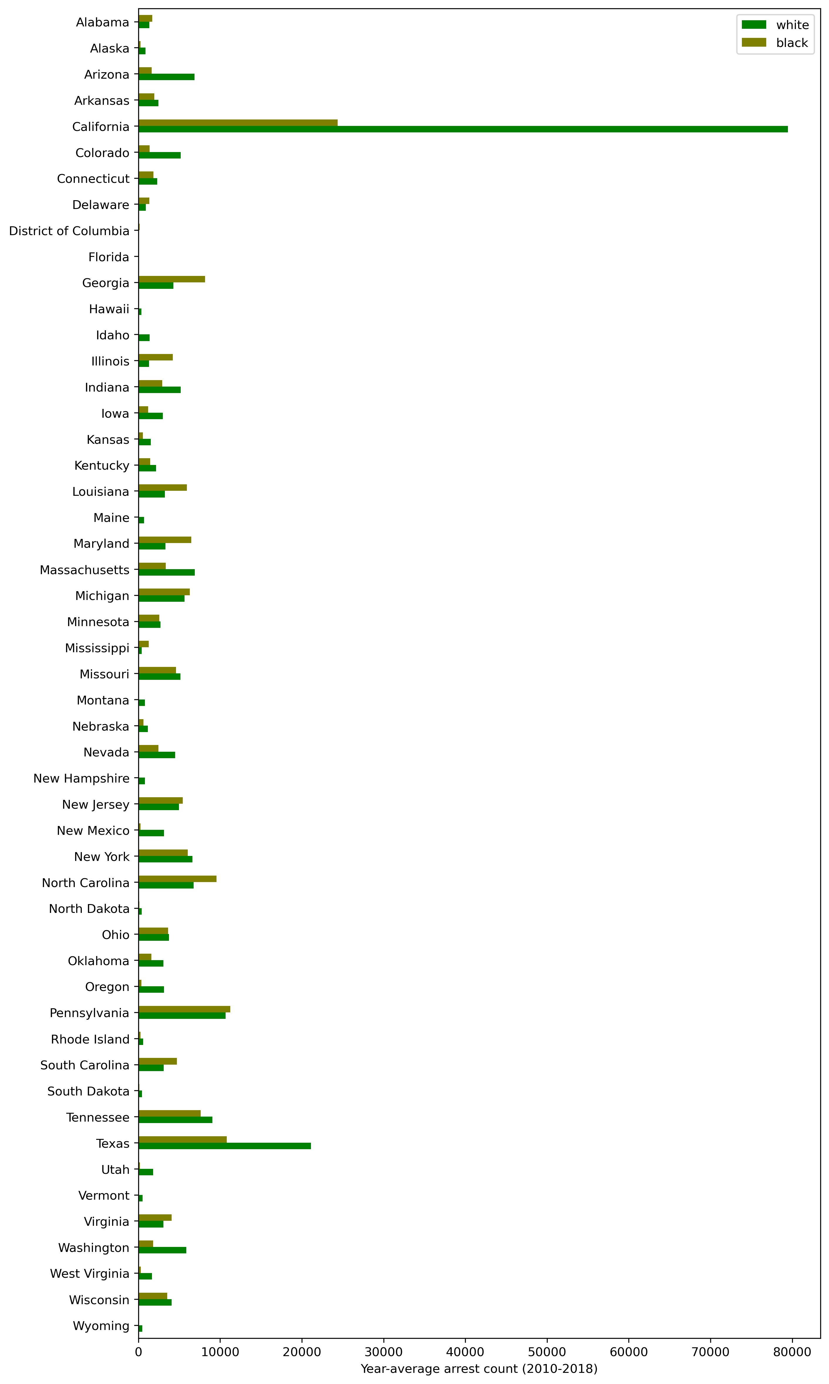
1. Absolute arrest counts
plt = df_arrests_2010_2018_agg[['white', 'black']].sort_index(ascending=False).\
                   plot.barh(color=['g', 'olive'], figsize=(10, 20))
plt.set_ylabel('')
plt.set_xlabel('Year-average arrest count (2010-2018)')
Tall image

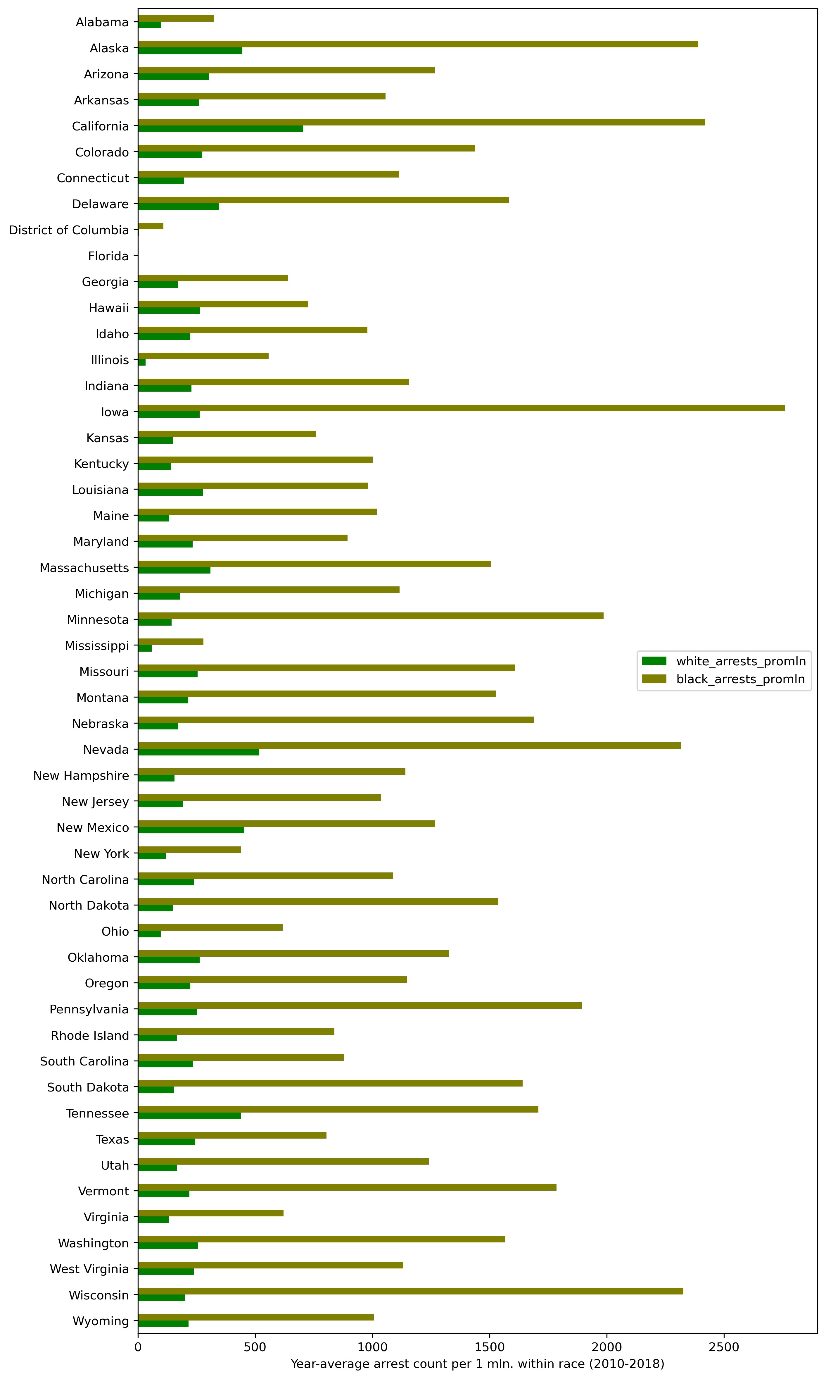
2. Arrest counts per million population (for each race)
plt = df_arrests_2010_2018_agg[['white_arrests_promln', 'black_arrests_promln']].\
          sort_index(ascending=False).plot.barh(color=['g', 'olive'], figsize=(10, 20))
plt.set_ylabel('')
plt.set_xlabel('Year-average arrest count per 1 mln. within race (2010-2018)')
Another tall image

What can we infer from this data?
First of all, we see that the number of arrests is affected by population — this is observed for both races.
Secondly, Whites get busted somewhat more often than Blacks in absolute figures. The 'somewhat' — because this rule isn't universal for all the states (exclusions are North Carolina, Georgia, Louisiana, etc.); at the same time, the difference is but slight in most states, except a few (like California, Texas, Colorado, Massachusetts and a few others).
Last but not least, Blacks get arrested much more often in all the states in per capita values.
Let's back these observations by numbers.
Difference between the average White and Black arrest counts:
df_arrests_2010_2018['white'].mean() / df_arrests_2010_2018['black'].mean()
— we get 1.56. That is, the observed 9 years saw on average one and a half times more Whites being arrested than Blacks.
Then in per capita values:
df_arrests_2010_2018['white_arrests_promln'].mean() /
                                     df_arrests_2010_2018['black_arrests_promln'].mean()
— the ratio is 0.183. That is, a Black person is on average 5.5 times more likely to get arrested than a White person.
Thus, the previous conclusion of higher criminality among Blacks (compared to Whites) is confirmed by the arrest data for all the states of the USA.
To understand how race and criminality are connected with lethal force victims, let's merge the two datasets.
First, we prepare the use-of-force data with the victims' race details:
df_fenc_agg_states1 = df_fenc.merge(df_state_names, how='inner',
                                          left_on='State', right_on='state_abbr')
df_fenc_agg_states1.fillna(0, inplace=True)
df_fenc_agg_states1 = df_fenc_agg_states1.rename(columns={
                                          'state_name_x': 'state_name', 'Year': 'year'})
df_fenc_agg_states1 = df_fenc_agg_states1.loc[df_fenc_agg_states1['year'].\
                                  between(2000, 2018), ['year', 'Race', 'state_name', 'UOF']]
df_fenc_agg_states1 = df_fenc_agg_states1.groupby(['year', 'state_name', 'Race'])['UOF'].\
                                    count().unstack().reset_index()
df_fenc_agg_states1 = df_fenc_agg_states1.rename(columns={
                                   'Black': 'black_uof', 'White': 'white_uof'})
df_fenc_agg_states1 = df_fenc_agg_states1.fillna(0).astype({
                                    'black_uof': 'uint32', 'white_uof': 'uint32'})
Resulting UOF dataset
| Race | year | state_name | black_uof | white_uof |
|---|---|---|---|---|
| 0 | 2000 | Alabama | 4 | 3 |
| 1 | 2000 | Alaska | 0 | 2 |
| 2 | 2000 | Arizona | 0 | 11 |
| 3 | 2000 | Arkansas | 1 | 3 |
| 4 | 2000 | California | 19 | 78 |
| ... | ... | ... | ... | ... |
| 907 | 2018 | Virginia | 11 | 7 |
| 908 | 2018 | Washington | 0 | 24 |
| 909 | 2018 | West Virginia | 2 | 5 |
| 910 | 2018 | Wisconsin | 3 | 7 |
| 911 | 2018 | Wyoming | 0 | 4 |
Then we're merging it with the arrest data:
df_arrests_fenc = df_arrests.merge(df_fenc_agg_states1,
                    on=['state_name', 'year'])
df_arrests_fenc = df_arrests_fenc.rename(columns={
                   'white': 'white_arrests', 'black': 'black_arrests'})
Example data for 2017
| year | state | black_arrests | white_arrests | state_name | black_uof | white_uof | |
|---|---|---|---|---|---|---|---|
| 15 | 2017 | AK | 266 | 859 | Alaska | 2 | 3 |
| 34 | 2017 | AL | 3098 | 2509 | Alabama | 7 | 17 |
| 53 | 2017 | AR | 2092 | 2674 | Arkansas | 6 | 7 |
| 72 | 2017 | AZ | 2431 | 7829 | Arizona | 6 | 43 |
| 91 | 2017 | CA | 24937 | 80367 | California | 25 | 137 |
| 110 | 2017 | CO | 1781 | 6079 | Colorado | 2 | 27 |
| 127 | 2017 | CT | 1687 | 2114 | Connecticut | 1 | 5 |
| 140 | 2017 | DE | 1198 | 782 | Delaware | 4 | 3 |
| 159 | 2017 | GA | 7747 | 4171 | Georgia | 15 | 21 |
| 173 | 2017 | HI | 88 | 419 | Hawaii | 0 | 1 |
| 192 | 2017 | IA | 1400 | 3524 | Iowa | 1 | 5 |
| 210 | 2017 | ID | 61 | 1423 | Idaho | 0 | 6 |
| 229 | 2017 | IL | 2847 | 947 | Illinois | 13 | 11 |
| 248 | 2017 | IN | 3565 | 4300 | Indiana | 9 | 13 |
| 267 | 2017 | KS | 585 | 1651 | Kansas | 3 | 10 |
| 286 | 2017 | KY | 1481 | 2035 | Kentucky | 1 | 18 |
| 305 | 2017 | LA | 5875 | 2284 | Louisiana | 13 | 5 |
| 324 | 2017 | MA | 2953 | 6089 | Massachusetts | 1 | 4 |
| 343 | 2017 | MD | 6662 | 3371 | Maryland | 8 | 5 |
| 361 | 2017 | ME | 89 | 675 | Maine | 1 | 8 |
| 380 | 2017 | MI | 6149 | 5459 | Michigan | 6 | 7 |
| 399 | 2017 | MN | 2513 | 2681 | Minnesota | 1 | 7 |
| 418 | 2017 | MO | 4571 | 5007 | Missouri | 13 | 20 |
| 437 | 2017 | MS | 1266 | 409 | Mississippi | 7 | 10 |
| 455 | 2017 | MT | 50 | 915 | Montana | 0 | 3 |
| 474 | 2017 | NC | 8177 | 5576 | North Carolina | 9 | 14 |
| 501 | 2017 | NE | 80 | 578 | Nebraska | 0 | 1 |
| 516 | 2017 | NH | 113 | 817 | New Hampshire | 0 | 3 |
| 535 | 2017 | NJ | 4859 | 4136 | New Jersey | 9 | 6 |
| 554 | 2017 | NM | 205 | 2094 | New Mexico | 0 | 20 |
| 573 | 2017 | NV | 2695 | 4657 | Nevada | 3 | 12 |
| 592 | 2017 | NY | 5923 | 6633 | New York | 7 | 9 |
| 611 | 2017 | OH | 4472 | 3882 | Ohio | 11 | 23 |
| 630 | 2017 | OK | 1638 | 2872 | Oklahoma | 3 | 20 |
| 649 | 2017 | OR | 453 | 3222 | Oregon | 2 | 9 |
| 668 | 2017 | PA | 10123 | 10191 | Pennsylvania | 7 | 17 |
| 681 | 2017 | RI | 315 | 633 | Rhode Island | 0 | 1 |
| 700 | 2017 | SC | 4645 | 2964 | South Carolina | 3 | 10 |
| 712 | 2017 | SD | 124 | 537 | South Dakota | 0 | 2 |
| 731 | 2017 | TN | 6654 | 8496 | Tennessee | 4 | 24 |
| 750 | 2017 | TX | 11493 | 20911 | Texas | 18 | 56 |
| 769 | 2017 | UT | 199 | 1964 | Utah | 1 | 5 |
| 788 | 2017 | VA | 4283 | 3247 | Virginia | 8 | 17 |
| 804 | 2017 | VT | 75 | 626 | Vermont | 0 | 1 |
| 823 | 2017 | WA | 1890 | 5804 | Washington | 8 | 27 |
| 842 | 2017 | WV | 350 | 1705 | West Virginia | 1 | 10 |
| 856 | 2017 | WY | 36 | 549 | Wyoming | 0 | 1 |
| 872 | 2017 | DC | 135 | 8 | District of Columbia | 1 | 1 |
| 890 | 2017 | WI | 3604 | 4106 | Wisconsin | 6 | 15 |
| 892 | 2017 | FL | 12 | 7 | Florida | 19 | 43 |
OK, time to calculate the correlation coefficients between arrests and lethal force fatalities, as we did before:
df_corr = df_arrests_fenc.loc[:, ['white_arrests', 'black_arrests',
                      'white_uof', 'black_uof']].corr(method='pearson').iloc[:2, 2:]
df_corr.style.background_gradient(cmap='PuBu')
| white_uof | black_uof | |
|---|---|---|
| white_arrests | 0.872766 | 0.622167 |
| black_arrests | 0.702350 | 0.766852 |
Again we've produced quite good correlations: 0.87 for Whites and 0.77 for Blacks. It's curious that these values are very close to those we obtained for All Offenses in the previous part of the article (0.88 for Whites and 0.72 for Blacks).
What about our 'offender shootdown' index? Let's check:
df_arrests_fenc['white_uof_by_arr'] = df_arrests_fenc['white_uof'] /
                            df_arrests_fenc['white_arrests']
df_arrests_fenc['black_uof_by_arr'] = df_arrests_fenc['black_uof'] /
                            df_arrests_fenc['black_arrests']
df_arrests_fenc.replace([np.inf, -np.inf], np.nan, inplace=True)
df_arrests_fenc.fillna({'white_uof_by_arr': 0, 'black_uof_by_arr': 0}, inplace=True)
To see how this index is distributed geographically, let's take the 2018 data point:
plt = df_arrests_fenc.loc[df_arrests_fenc['year'] == 2018,
                             ['state_name', 'white_uof_by_arr', 'black_uof_by_arr']].\
                             sort_values(by='state_name', ascending=False).\
                             plot.barh(x='state_name', color=['g', 'olive'], figsize=(10, 20))
plt.set_ylabel('')
plt.set_xlabel('Ratio of UOF victims to violent crimes (2018)')
Tall image again

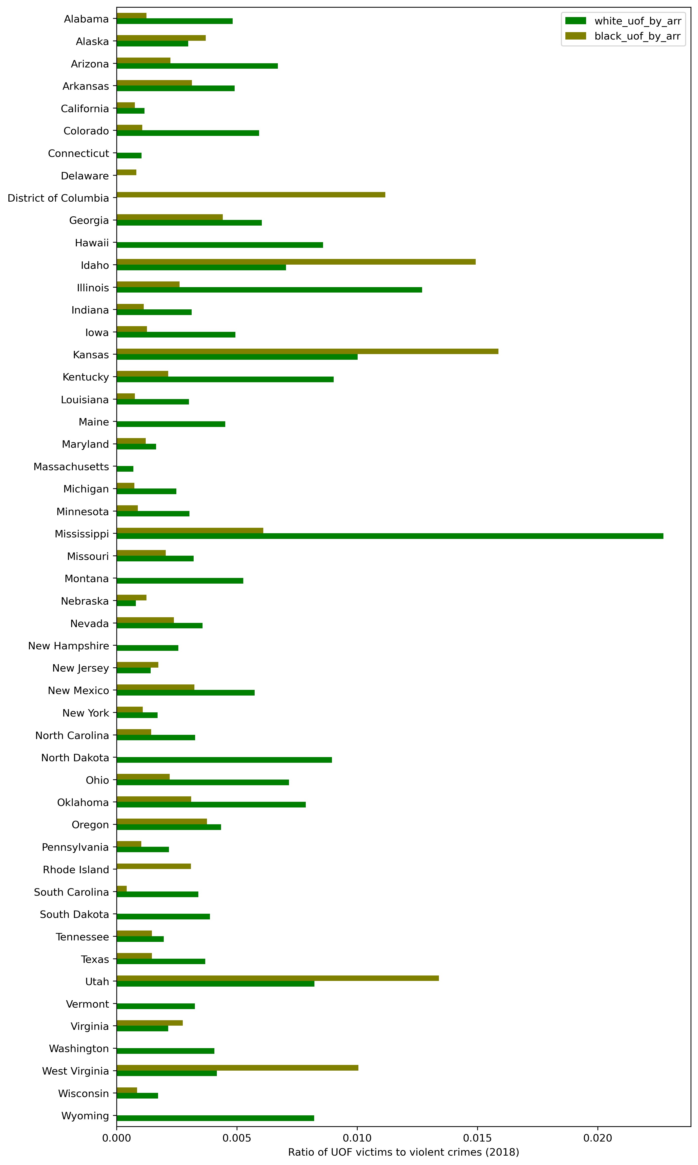
The index for Whites is greater in most states, with some exclusions (Utah, West Virginia, Kansas, Idaho, and District Columbia).
Let's compare the values for Whites and Blacks averaged for all the states:
plt = df_arrests_fenc.loc[:, ['white_uof_by_arr', 'black_uof_by_arr']].\
                                   mean().plot.bar(color=['g', 'olive'])
plt.set_ylabel('Ratio of UOF victims to violent crimes (2018)')
plt.set_xticklabels(['White', 'Black'], rotation=0)
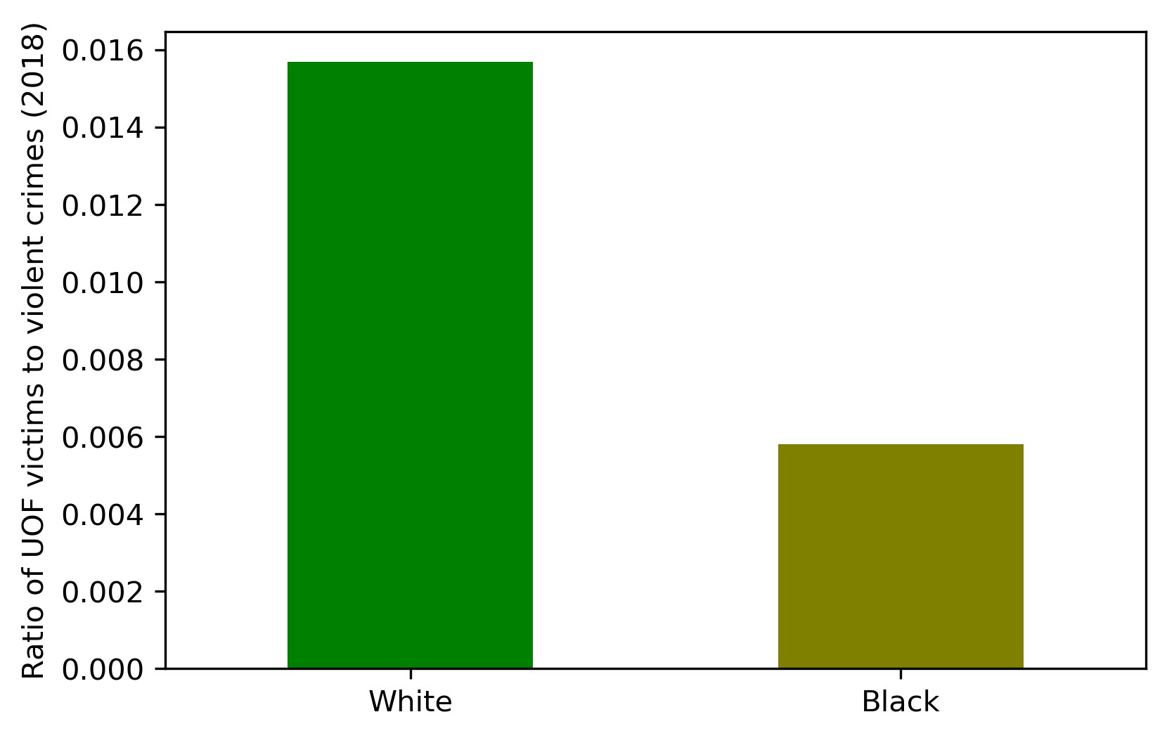
The index is 2.5 times greater for Whites than for Blacks. If this index really says something, it means that a White criminal is on average 2.5 times more likely to meet death from the police than a Black criminal. Of course, this index varies much from state to state: for example, in Idaho a Black criminal is twice as likely to become a law enforcement victim, whereas in Mississippi — four times less likely.
Well, that's it really. Time to summarize our research.
Conclusions
- In the US, criminality is a function of population. The most 'criminal' states that we are used to watching movies or read about are simply the most populated. When analyzing per capita crime rates, the top positions are taken by some quite unexpected states like Alaska, District Columbia (with Washington City) and New Mexico.
- Southern states are on average more criminal than Northern states (in per capita crime values).
- Per capita crimes and arrests are unevenly distributed among the US white and black populations: black persons commit 3 times more crimes and are 5 times more often arrested than white persons.
- A black person is on average 2.5 times more likely to get killed in an encounter with law enforcement than a white person.
- Lethal force fatalities correlate well with criminality: the higher the crime rate, the more people get killed by the police. This correlation holds true for most states and for both races, although it is somewhat more pronounced among the white population. This is also confirmed by the difference in the victim-to-crime ratio between the races: white criminals are more likely to get killed by the police.
As a final word, I'd like to say thanks to my readers for their valuable comments and advice.
P.S. In a future (separate) article I am planning to continue analyzing crime and its connection with race in the US. We can first look into hate crimes and then discuss the law enforcement / offender interfaces from a reversed point of view, investigating line-of-duty fatalities among US police officers. I'd appreciate if you let me know in the comments if this subject is of interest.
