Queries in PostgreSQL. Sort and merge

In the previous articles, we have covered query execution stages, statistics, sequential and index scan, and two of the three join methods: nested loop and hash join.

This last article of the series will cover the merge algorithm and sorting. I will also demonstrate how the three join methods compare against each other.

Merge join

The merge join algorithm takes two data sets that are sorted by the merge key and returns an ordered output. The input data sets may be pre-sorted by an index scan or be sorted explicitly.

Merging sorted sets

Below is an example of a merge join. Note the Merge Join node in the plan.

EXPLAIN (costs off) SELECT *
FROM tickets t
  JOIN ticket_flights tf ON tf.ticket_no = t.ticket_no
ORDER BY t.ticket_no;

                           QUERY PLAN
−−−−−−−−−−−−−−−−−−−−−−−−−−−−−−−−−−−−−−−−−−−−−−−−−−−−−−−−−−−−−−−−
 Merge Join
   Merge Cond: (t.ticket_no = tf.ticket_no)
   −> Index Scan using tickets_pkey on tickets t
   −> Index Scan using ticket_flights_pkey on ticket_flights tf
(4 rows)

Here, the optimizer selected this join method because it returns the output ordered by the key specified under the ORDER BY clause. When selecting a plan, the optimizer considers the ordering of the input and tries to avoid sorting altogether whenever possible. In addition to that, the resulting output can be used as an input for another merge join as long as the ordering stays intact:

EXPLAIN (costs off) SELECT *
FROM tickets t
  JOIN ticket_flights tf ON t.ticket_no = tf.ticket_no
  JOIN boarding_passes bp ON bp.ticket_no = tf.ticket_no
                         AND bp.flight_id = tf.flight_id
ORDER BY t.ticket_no;

                             QUERY PLAN
−−−−−−−−−−−−−−−−−−−−−−−−−−−−−−−−−−−−−−−−−−−−−−−−−−−−−−−−−−−−−−−−−−−−−
 Merge Join
   Merge Cond: (tf.ticket_no = t.ticket_no)
   −> Merge Join
       Merge Cond: ((tf.ticket_no = bp.ticket_no) AND (tf.flight_...
       −> Index Scan using ticket_flights_pkey on ticket_flights tf
       −> Index Scan using boarding_passes_pkey on boarding_passe...
  −> Index Scan using tickets_pkey on tickets t
(7 rows)

The ticket_flights and boarding_passes tables are merged first. The tables have a composite primary key (ticket_no, flight_id), so the output is ordered by these two columns. The resulting set of rows is then merged with the tickets table, which is ordered by ticket_no.

The merge is completed in one pass over the two data sets and does not require any extra memory. The algorithm uses two pointers, which point at the current (or initially, the first) rows of the two sets.

If the keys of the current rows don't match, one of the pointers (the one that points at the row with the lower key) moves one step forward. This repeats until a match is found. Matching rows are returned to the parent node, and the inner set pointer moves one step forward. The algorithm repeats until it reaches the end of either set.

This specific algorithm can handle duplicate keys in the inner but not in the outer set. An additional step is introduced to fix that: whenever the outer pointer moves but the key remains the same, the inner pointer is returned to the first row that matches the key. This way, every outer set row will be matched with all inner set rows that have the same key.

There is another variation of the algorithm that can perform outer joins, but it is based on the same principle.

The merge join is designed to work with the equity operator, so it supports only equijoins (but there is an effort to support other comparison operators as well).

Cost estimation. Consider the example from before:

EXPLAIN SELECT *
FROM tickets t
  JOIN ticket_flights tf ON tf.ticket_no = t.ticket_no
ORDER BY t.ticket_no;

                          QUERY PLAN
−−−−−−−−−−−−−−−−−−−−−−−−−−−−−−−−−−−−−−−−−−−−−−−−−−−−−−−−−−−−−−−−
 Merge Join  (cost=0.99..822358.66 rows=8391852 width=136)
   Merge Cond: (t.ticket_no = tf.ticket_no)
   −> Index Scan using tickets_pkey on tickets t
       (cost=0.43..139110.29 rows=2949857 width=104)
   −> Index Scan using ticket_flights_pkey on ticket_flights tf
       (cost=0.56..570975.58 rows=8391852 width=32)
(6 rows)

Initially, the startup cost includes at least the startup costs of the child nodes.

In addition to that, you more often than not will have to scan at least some fraction of both data sets before the first match is found. To estimate this fraction, you can use a histogram to compare the minimal join keys in both sets. In this case, however, the range of ticket numbers in both tables is the same.

The total cost of the node is the sum of the data retrieval cost from its children and the data processing cost.

Because the algorithm stops when it reaches the end of either of the two sets (except when performing an outer join, of course), a fraction of the second set may remain unscanned. You can estimate the size of that fraction by comparing the maximum keys of both sets. In this case, both our sets will be scanned fully, so we include the full total costs of the child nodes into the parent's total cost.

Additionally, duplicate keys may cause some of the inner set rows to be scanned multiple times. The number of repeat scans is proportional to the difference between the join result and the inner set cardinality.

Here, these cardinalities are the same, which means there are no duplicates.

The data processing cost comprises key comparisons and result output. The number of comparisons could be estimated by adding up the cardinalities of both sets and the number of repeat outer set row scans. The cost of one comparison is estimated as cpu_operator_cost, the row output cost as cpu_tuple_cost.

Now we can calculate the join cost for our example:

SELECT 0.43 + 0.56 AS startup,
  round((
    139110.29 + 570975.58 +
    current_setting('cpu_tuple_cost')::real * 8391852 +
    current_setting('cpu_operator_cost')::real * (2949857 + 8391852)
)::numeric, 2) AS total;

 startup |   total
−−−−−−−−−+−−−−−−−−−−−
    0.99 | 822358.66
(1 row)

Parallel mode

The merge join algorithm can be used in a parallelized plan.

The workers can scan the outer set in parallel, but each worker scans the inner set individually.

Here's an example of a parallel plan with a merge join:

SET enable_hashjoin = off;
EXPLAIN (costs off)
SELECT count(*), sum(tf.amount)
FROM tickets t
  JOIN ticket_flights tf ON tf.ticket_no = t.ticket_no;

                             QUERY PLAN
−−−−−−−−−−−−−−−−−−−−−−−−−−−−−−−−−−−−−−−−−−−−−−−−−−−−−−−−−−−−−−−−−−−−−
 Finalize Aggregate
   −> Gather
       Workers Planned: 2
       −> Partial Aggregate
           −> Merge Join
               Merge Cond: (tf.ticket_no = t.ticket_no)
               −> Parallel Index Scan using ticket_flights_pkey o...
               −> Index Only Scan using tickets_pkey on tickets t
(8 rows)

Full and right outer joins are not supported in this mode.

Modifications

The merge join supports all logical join types. The only limitation is that for full and right outer joins the join condition must be a valid expression for the merge operation (outer column equals inner column or column equals constant). For other logical join types, any non-mergejoinable conditions are applied to the output after the merging is complete, but it's impossible to do so for full and right outer joins.

Below is an example of a full merge join:

EXPLAIN (costs off) SELECT *
FROM tickets t
  FULL JOIN ticket_flights tf ON tf.ticket_no = t.ticket_no
ORDER BY t.ticket_no;

                             QUERY PLAN
−−−−−−−−−−−−−−−−−−−−−−−−−−−−−−−−−−−−−−−−−−−−−−−−−−−−−−−−−−−−−−−−−−−−
 Sort
   Sort Key: t.ticket_no
   −> Merge Full Join
       Merge Cond: (t.ticket_no = tf.ticket_no)
       −> Index Scan using tickets_pkey on tickets t
       −> Index Scan using ticket_flights_pkey on ticket_flights tf
(6 rows)

Inner and left outer merge joins preserve the ordering. Full and right outer joins do not, because NULL values that may appear among the data will break the ordering. This is where the Sort node comes in to reorder the output. It increases the cost, making the hash join a more attractive alternative, so we had to explicitly disable it for the demonstration.

In the next example, however, the hash join is selected anyway because a full join with non-mergejoinable conditions cannot be done in any other way.

EXPLAIN (costs off) SELECT *
FROM tickets t
  FULL JOIN ticket_flights tf ON tf.ticket_no = t.ticket_no
                             AND tf.amount > 0
ORDER BY t.ticket_no;

                  QUERY PLAN
−−−−−−−−−−−−−−−−−−−−−−−−−−−−−−−−−−−−−−−−−−−−−−−
 Sort
   Sort Key: t.ticket_no
   −> Hash Full Join
       Hash Cond: (tf.ticket_no = t.ticket_no)
       Join Filter: (tf.amount > '0'::numeric)
       −> Seq Scan on ticket_flights tf
       −> Hash
           −> Seq Scan on tickets t
(8 rows)

RESET enable_hashjoin;

Sorting

If either of the sets (or both) isn't ordered by the join key, it must be sorted before merging. This necessary sorting is done under the Sort node in the plan.

EXPLAIN (costs off)
SELECT *
FROM flights f
  JOIN airports_data dep ON f.departure_airport = dep.airport_code
ORDER BY dep.airport_code;

                       QUERY PLAN
−−−−−−−−−−−−−−−−−−−−−−−−−−−−−−−−−−−−−−−−−−−−−−−−−−−−−−−−
 Merge Join
   Merge Cond: (f.departure_airport = dep.airport_code)
   −> Sort
       Sort Key: f.departure_airport
       −> Seq Scan on flights f
   −> Sort
       Sort Key: dep.airport_code
       −> Seq Scan on airports_data dep
(8 rows)

The sorting algorithm itself is universal. It can be invoked by an ORDER BY clause by itself or within a window function:

EXPLAIN (costs off)
SELECT flight_id,
  row_number() OVER (PARTITION BY flight_no ORDER BY flight_id)
FROM flights f;

              QUERY PLAN
−−−−−−−−−−−−−−−−−−−−−−−−−−−−−−−−−−−−−−
 WindowAgg
   −> Sort
       Sort Key: flight_no, flight_id
       −> Seq Scan on flights f
(4 rows)

Here, the WindowAgg node calculates the window function over a data set pre-sorted by the Sort node.

The planner has an arsenal of sorting modes to choose from. The example above showcases two of those (Sort Method). As always, you can dig in for more details with EXPLAIN ANALYZE:

EXPLAIN (analyze,costs off,timing off,summary off)
SELECT *
FROM flights f
  JOIN airports_data dep ON f.departure_airport = dep.airport_code
ORDER BY dep.airport_code;

                            QUERY PLAN
−−−−−−−−−−−−−−−−−−−−−−−−−−−−−−−−−−−−−−−−−−−−−−−−−−−−−−−−−−−−−−−−−−
 Merge Join (actual rows=214867 loops=1)
   Merge Cond: (f.departure_airport = dep.airport_code)
   −> Sort (actual rows=214867 loops=1)
       Sort Key: f.departure_airport
       Sort Method: external merge Disk: 17136kB
       −> Seq Scan on flights f (actual rows=214867 loops=1)
   −> Sort (actual rows=104 loops=1)
       Sort Key: dep.airport_code
       Sort Method: quicksort Memory: 52kB
       −> Seq Scan on airports_data dep (actual rows=104 loops=1)
(10 rows)

Quicksort

If the data to be sorted fits into the allowed memory (work_mem) completely, then the good old Quicksort algorithm is used. You can find its description on the first pages of any computer science textbook, so I will not repeat it here.

For the implementation, the sorting is done by a specific component that selects the most appropriate algorithm for the task.

Cost estimation. Let's look at how the algorithm sorts a small table:

EXPLAIN SELECT *
FROM airports_data
ORDER BY airport_code;

                             QUERY PLAN
−−−−−−−−−−−−−−−−−−−−−−−−−−−−−−−−−−−−−−−−−−−−−−−−−−−−−−−−−−−−−−−−−−−−−
 Sort  (cost=7.52..7.78 rows=104 width=145)
   Sort Key: airport_code
   −> Seq Scan on airports_data  (cost=0.00..4.04 rows=104 width=...
(3 rows)

The complexity of sorting n values is O(n log₂n). One comparison operation costs twice the value of cpu_operator_cost. You need to scan and sort the whole set to get a result, so the startup sorting cost will include both the comparison operations cost and the total cost of the child node.

The total sorting cost will include, in addition to that, the processing cost for each row of the Sort node output, estimated as cpu_operator_cost per row (instead of the default cpu_tuple_cost because it is cheap).

So, the sorting cost for the example above would be calculated like this:

WITH costs(startup) AS (
  SELECT 4.04 + round((
    current_setting('cpu_operator_cost')::real * 2 *
      104 * log(2, 104)
  )::numeric, 2)
)
SELECT startup,
  startup + round((
    current_setting('cpu_operator_cost')::real * 104
  )::numeric, 2) AS total
FROM costs;

 startup | total
−−−−−−−−−+−−−−−−−
    7.52 | 7.78
(1 row)

Top-N heapsort

A top-N heapsort is something you do when you want just a part of a set sorted (up to a certain LIMIT) instead of the whole set. More precisely, this algorithm is used when the LIMIT will filter out at least half of the input rows, or when the input does not fit into the memory, but the output does.

EXPLAIN (analyze, timing off, summary off) SELECT *
FROM seats
ORDER BY seat_no
LIMIT 100;

                            QUERY PLAN
−−−−−−−−−−−−−−−−−−−−−−−−−−−−−−−−−−−−−−−−−−−−−−−−−−−−−−−−−−−−−−−−−−−
 Limit  (cost=72.57..72.82 rows=100 width=15)
   (actual rows=100 loops=1)
   −> Sort  (cost=72.57..75.91 rows=1339 width=15)
       (actual rows=100 loops=1)
       Sort Key: seat_no
       Sort Method: top−N heapsort Memory: 33kB
       −> Seq Scan on seats  (cost=0.00..21.39 rows=1339 width=15)
           (actual rows=1339 loops=1)
(8 rows)

In order to find the k highest (lowest) values out of n, the algorithm first creates a data structure called a heap and adds k first rows into it. Then it continues adding rows into the heap one by one, but after each one, it expels one lowest (highest) value from the heap. When it runs out of new rows to add, the heap is left with the k highest or lowest values.

The term heap here refers to a specific data structure and should not be confused with database tables, which often go by the same name.

Cost estimation. The algorithm complexity is O(nlog₂k), but each operation costs more compared to Quicksort, so the cost calculation formula uses n log₂2k as an estimate.

WITH costs(startup) AS (
  SELECT 21.39 + round((
    current_setting('cpu_operator_cost')::real * 2 *
      1339 * log(2, 2 * 100)
  )::numeric, 2)
)
SELECT startup,
  startup + round((
    current_setting('cpu_operator_cost')::real * 100
  )::numeric, 2) AS total
FROM costs;

 startup | total
−−−−−−−−−+−−−−−−−
   72.57 | 72.82
(1 row)

External sort

Whenever the executor discovers that the data set it's reading is too to be sorted in-memory, the Sort node switches into the external merge sort mode.

The rows scanned up to this point are sorted by Quicksort and dumped into a temporary file.

Then another batch of rows is scanned, sorted, and dumped, and so on. This repeats until all data is stored in a bunch of sorted files on disk.

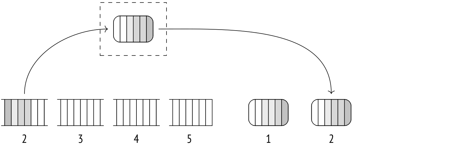
Then, the algorithm starts merging the files. The process is very similar to the merge join, although here more than two files can be merged at once.

The merging doesn't use up a lot of memory. In essence, as much as a single row's size per file is enough. The algorithm scans the first row of each file and stores them. Then, it selects the lowest (or the highest) value among the stored ones and returns it as an output. After that, it takes another row and puts it into the memory where the returned row was stored.

In practice, the rows are scanned not one by one, but in batches of 32 pages each, to save on I/O costs. The number of files merged at once is determined by the amount of available memory, but it's never less than six. It's also never more than 500, because algorithm efficiency suffers at high numbers of concurrently merged files.

If all temporary files can't be merged in a single iteration, the result of the first merge is dumped into its own temporary file. Each iteration increases the amount of data being read from and written to disk, slowing down the process, so it's beneficial to have as much memory as possible for external merge sort to run efficiently.

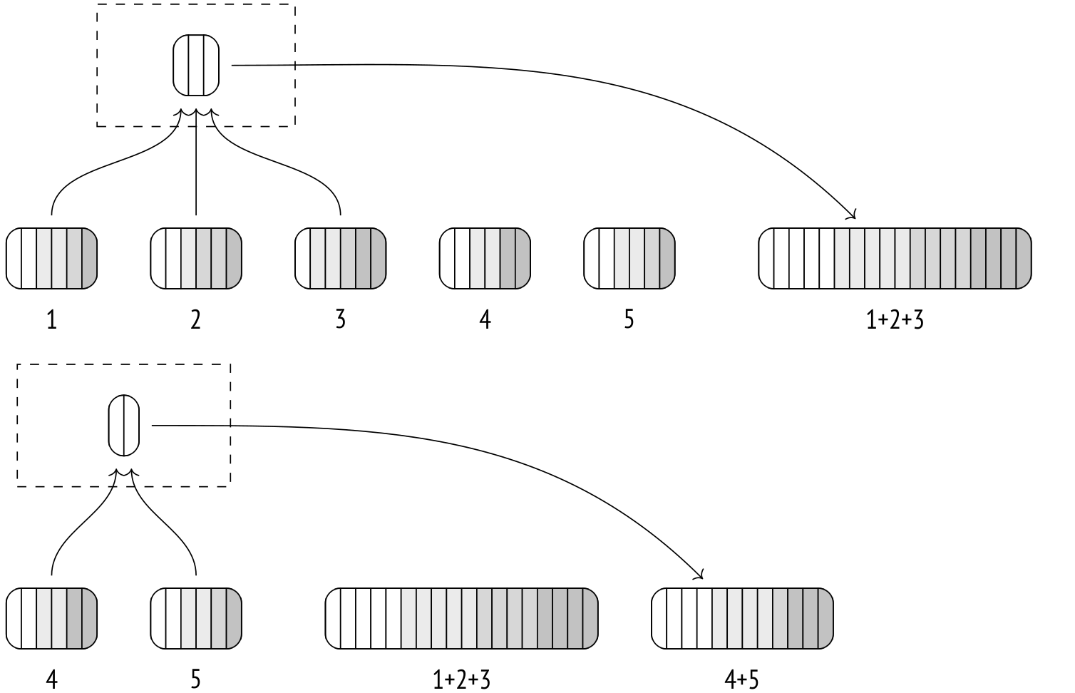
The second iteration takes the temporary files produced by the first iteration and repeats the process.

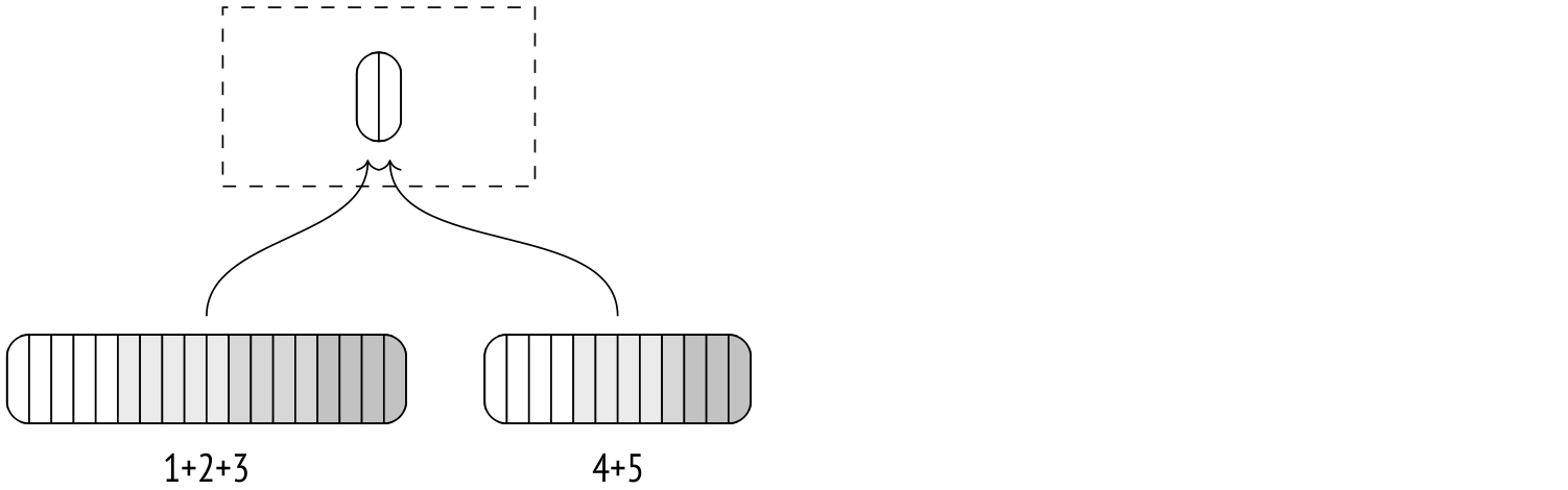
The final merge is usually postponed and only performed when the parent node pulls the data.

Let's use EXPLAIN ANALYZE to see how much disk space the sorting used up. You can also check out the buffer usage statistics for the temporary files (temp read and written) by using the buffers option. The numbers for buffers read and written will be about the same and, converted into KB, will match the Disk value in the plan.

EXPLAIN (analyze, buffers, costs off, timing off, summary off)
SELECT *
FROM flights
ORDER BY scheduled_departure;

                            QUERY PLAN
−−−−−−−−−−−−−−−−−−−−−−−−−−−−−−−−−−−−−−−−−−−−−−−−−−−−−−−−−−−−−−−−−−
 Sort (actual rows=214867 loops=1)
   Sort Key: scheduled_departure
   Sort Method: external merge Disk: 17136kB
   Buffers: shared hit=610 read=2017, temp read=2142 written=2150
   −> Seq Scan on flights (actual rows=214867 loops=1)
       Buffers: shared hit=607 read=2017
(6 rows)

There are more statistics about the temporary files to be found in the server log (with the parameter log_temp_buffers on).

Cost estimation. Let's look at the external merge sort plan again:

EXPLAIN SELECT *
FROM flights
ORDER BY scheduled_departure;

                             QUERY PLAN
−−−−−−−−−−−−−−−−−−−−−−−−−−−−−−−−−−−−−−−−−−−−−−−−−−−−−−−−−−−−−−−−−−−−−
 Sort  (cost=31883.96..32421.12 rows=214867 width=63)
   Sort Key: scheduled_departure
   −> Seq Scan on flights  (cost=0.00..4772.67 rows=214867 width=63)
(3 rows)

Here, the basic comparison cost is the same as in Quicksort, but there's also an I/O cost added on top. All input data is first dumped to disk, then read from disk for merging (multiple times, if there are too many individual files to be merged in one pass).

The volume of data written to disk depends on the number and size of rows in the input data set. In this example, the query pulls all the columns from the flights table, so the data size will be close to the table size, except it will not include any tuple headers and page metadata (2309 pages vs 2624). Here, one iteration is enough to sort the data.

The I/O operations (both reading and writing) are estimated to be sequential 3/4 of the time and random 1/4 of the time.

So in the end, the sorting cost will be calculated like this:

WITH costs(startup) AS (
  SELECT 4772.67 + round((
    current_setting('cpu_operator_cost')::real * 2 *
      214867 * log(2, 214867) +
    (current_setting('seq_page_cost')::real * 0.75 +
      current_setting('random_page_cost')::real * 0.25) *
    2 * 2309 * 1 -- one iteration
  )::numeric, 2)
)
SELECT startup,
  startup + round(( current_setting('cpu_operator_cost')::real * 214867
  )::numeric, 2) AS total
FROM costs;

 startup  |  total
−−−−−−−−−−+−−−−−−−−−−
 31883.96 | 32421.13
(1 row)

Incremental sort

Let's suppose you want to sort a set by keys K₁… K_m… K_n, and it's known that the set is already sorted by some of the first keys K₁… K_m. Then, you can save time by not sorting the entire set. Instead, you can split the set into groups, with each group containing only rows with the same K₁… K_m values (arranged consecutively) and then sort each group by the remaining keys K_m+1… K_n. This method is called incremental sort and it's made available in PostgreSQL 13 and above.

Incremental sort reduces the memory requirements by splitting the set into multiple smaller groups and also can start feeding the output group by group, without waiting for the whole set to be processed.

The actual implementation employs an additional optimization: while it separates larger chunks of rows into groups to be sorted individually, smaller subsets are put into one group and sorted together. This reduces the sorting startup overhead cost compared to the bare-bones algorithm.

The Incremental Sort node in the plan is where the sorting takes place:

EXPLAIN (analyze, costs off, timing off, summary off)
SELECT *
FROM bookings
ORDER BY total_amount, book_date;

                             QUERY PLAN
−−−−−−−−−−−−−−−−−−−−−−−−−−−−−−−−−−−−−−−−−−−−−−−−−−−−−−−−−−−−−−−−−−−−
 Incremental Sort (actual rows=2111110 loops=1)
   Sort Key: total_amount, book_date
   Presorted Key: total_amount
   Full−sort Groups: 2823 Sort Method: quicksort Average
   Memory: 30kB Peak Memory: 30kB
   Pre−sorted Groups: 2624 Sort Method: quicksort Average
   Memory: 3152kB Peak Memory: 3259kB
   −> Index Scan using bookings_total_amount_idx on bookings (ac...
(8 rows)

As evident from the plan, the set is pre-sorted by total_amount, being the output of an index scan against this column (Presorted Key). The EXPLAIN ANALYZE command also shows us the time it took to process the data. The Full-sort Groups value displays the number of rows that were clumped together and sorted regularly, and the Pre-sorted Groups shows the number of large groups that were incrementally sorted by the book_date column. In-memory Quicksort was used in both cases. The variation in the size of the groups is caused by the distribution of booking costs, which is non-uniform.

In PostgreSQL 14 and above, incremental sort also works with window functions:

EXPLAIN (costs off)
SELECT row_number() OVER (ORDER BY total_amount, book_date)
FROM bookings;

                           QUERY PLAN
−−−−−−−−−−−−−−−−−−−−−−−−−−−−−−−−−−−−−−−−−−−−−−−−−−−−−−−−−−−−−−−−−
 WindowAgg
   −> Incremental Sort
       Sort Key: total_amount, book_date
       Presorted Key: total_amount
       −> Index Scan using bookings_total_amount_idx on bookings
(5 rows)

Cost estimation. Incremental sort cost depends on the estimated number of groups and the estimated cost of sorting an average group (which we have covered before).

The startup cost shows the cost of sorting one (the first) group because that's enough for the node to begin output. The total cost includes the cost of sorting all the groups.

EXPLAIN SELECT *
FROM bookings
ORDER BY total_amount, book_date;

                             QUERY PLAN
−−−−−−−−−−−−−−−−−−−−−−−−−−−−−−−−−−−−−−−−−−−−−−−−−−−−−−−−−−−−−−−−−−−−−
 Incremental Sort  (cost=45.10..282293.40 rows=2111110 width=21)
   Sort Key: total_amount, book_date
   Presorted Key: total_amount
   −> Index Scan using bookings_total_amount_idx on bookings  (co...
(4 rows)

I'll skip the details of the calculation here.

Parallel mode

Sorting can be performed in parallel. That said, while the workers return their outputs sorted, the Gather node doesn't order them in any way, only appends the input in whatever order it comes in. To keep the rows ordered, another node is employed: Gather Merge.

EXPLAIN (analyze, costs off, timing off, summary off)
SELECT *
FROM flights
ORDER BY scheduled_departure
LIMIT 10;

                             QUERY PLAN
−−−−−−−−−−−−−−−−−−−−−−−−−−−−−−−−−−−−−−−−−−−−−−−−−−−−−−−−−−−−−−−−−−−−−
 Limit (actual rows=10 loops=1)
   −> Gather Merge (actual rows=10 loops=1)
       Workers Planned: 1
       Workers Launched: 1
       −> Sort (actual rows=8 loops=2)
           Sort Key: scheduled_departure
           Sort Method: top−N heapsort Memory: 27kB
           Worker 0: Sort Method: top−N heapsort Memory: 27kB
           −> Parallel Seq Scan on flights (actual rows=107434 lo...
(9 rows)

The Gather Merge node uses a binary heap to sort the rows coming in from workers. In essence, it just merges several sets of rows, much like the external merge sort, but there are some differences under the hood, one of them being that the Gather Merge node is optimized for working with a small, fixed number of data sources and for receiving rows one by one, without block I/O.

Cost estimation. The Gather Merge startup cost depends on the child node startup cost. As with the Gather node, there is also the worker processes startup cost, estimated as the parallel_setup_cost parameter value.

In addition to that, there is the binary heap building cost, which comprises sorting n items where n is the number of parallel workers, that is, n log₂n. The comparison operation cost is estimated as cpu_operator_cost times two. The resulting cost is usually insignificant because the number of workers is never that high.

The total cost then adds to that the data retrieval cost by the child node (performed by multiple workers) and the data output cost from the workers. The retrieval and output costs are estimated as parallel_tuple_cost per row plus 5% on account of possible delays.

Lastly, there is the binary heap update, which requires log₂n comparison operations plus auxiliary operations. Its cost is estimated as log N (2 cpu_operator_cost) + cpu_operator_cost per input row.

Here's another plan with a Gather Merge:

EXPLAIN SELECT amount, count(*)
FROM ticket_flights
GROUP BY amount;

                             QUERY PLAN
−−−−−−−−−−−−−−−−−−−−−−−−−−−−−−−−−−−−−−−−−−−−−−−−−−−−−−−−−−−−−−−−−−−−−
 Finalize GroupAggregate  (cost=123399.62..123485.00 rows=337 wid...
   Group Key: amount
   −> Gather Merge  (cost=123399.62..123478.26 rows=674 width=14)
       Workers Planned: 2
       −> Sort  (cost=122399.59..122400.44 rows=337 width=14)
           Sort Key: amount
           −> Partial HashAggregate  (cost=122382.07..122385.44 r...
               Group Key: amount
               −> Parallel Seq Scan on ticket_flights  (cost=0.00...
(9 rows)

Note that the workers here perform a partial hash aggregation before passing the results to the Sort node. This is efficient because aggregation cuts down on the number of rows. Then, the Sort node passes the output to the leader process to be assembled by the Gather Merge node. The final aggregation make use of a sorted list of values instead of hashing.

In this example, there are three parallel processes (including the leader), so the Gather Merge cost would be calculated as follows:

WITH costs(startup, run) AS (
  SELECT round((
    -- starting up the processes
    current_setting('parallel_setup_cost')::real +
    -- building the heap
    current_setting('cpu_operator_cost')::real * 2 * 3 * log(2, 3)
  )::numeric, 2),
  round((
    -- transmitting the rows
    current_setting('parallel_tuple_cost')::real * 1.05 * 674 +
    -- updating the heap
    current_setting('cpu_operator_cost')::real * 2 * 674 * log(2, 3) +
    current_setting('cpu_operator_cost')::real * 674
  )::numeric, 2)
)
SELECT 122399.59 + startup AS startup,
  122400.44 + startup + run AS total
FROM costs;

  startup  |   total
−−−−−−−−−−−+−−−−−−−−−−−
 123399.61 | 123478.26
(1 row)

Grouping and distinct values

The example from before shows that grouping values for aggregation (and removal of duplicate values) can be done both by hashing as well as by sorting. In a sorted list, groups of duplicate values can be found in a single pass.

A simple node called Unique performs the task of selecting distinct values from a given list:

EXPLAIN (costs off) SELECT DISTINCT book_ref
FROM bookings
ORDER BY book_ref;

                        QUERY PLAN
−−−−−−−−−−−−−−−−−−−−−−−−−−−−−−−−−−−−−−−−−−−−−−−−−−−−−−−−−−
 Result
   −> Unique
       −> Index Only Scan using bookings_pkey on bookings
(3 rows)

The aggregation itself is performed under the GroupAggregate node.

EXPLAIN (costs off) SELECT book_ref, count(*)
FROM bookings
GROUP BY book_ref
ORDER BY book_ref;

                      QUERY PLAN
−−−−−−−−−−−−−−−−−−−−−−−−−−−−−−−−−−−−−−−−−−−−−−−−−−−−−−
 GroupAggregate
   Group Key: book_ref
   −> Index Only Scan using bookings_pkey on bookings
(3 rows)

In parallel plans, this node will be replaced by Partial GroupAggregate, and the aggregation will be finalized under Finalize GroupAggregate.

In PostgreSQL 10 and above, both hashing and sorting can be used by the same node when grouping is performed over multiple sets (under GROUPING SETS, CUBE, and ROLLUP clauses). The details of the algorithm are too complicated to cover within the scope of this article, but we can have a look at an example instead. In this plan, grouping is performed over three different columns, and memory is limited.

SET work_mem = '64kB';
EXPLAIN (costs off)
SELECT count(*)
FROM flights
GROUP BY GROUPING SETS (aircraft_code, flight_no, departure_airport);

          QUERY PLAN
−−−−−−−−−−−−−−−−−−−−−−−−−−−−−−−
 MixedAggregate
   Hash Key: departure_airport
   Group Key: aircraft_code
   Sort Key: flight_no
     Group Key: flight_no
   −> Sort
       Sort Key: aircraft_code
       −> Seq Scan on flights
(8 rows)

The aggregate node, MixedAggregate, receives a set of rows pre-sorted by aircraft_code.

First, the set is scanned, and the rows are grouped by aircraft_code (Group Key). As the rows are being scanned, they are reordered by flight_no (either by Quicksort in memory (if sufficient) or by external sort on disk, just like the Sort node does it). At the same time, the rows are recorded into a hash table under the key departure_airport (either in-memory or in temporary files on disk, just like with the HashAggregate).

Next, the set that just got sorted by flight_no is scanned and grouped by the same key (Sort Key and the nested Group Key). If grouping by another column were required, the rows would have been reordered accordingly at this stage.

Finally, the hash table from the first step is scanned and the values are grouped by departure_airport (Hash Key).

Comparison of join methods

There are three methods that can be used to join two data sets, each with its own advantages and disadvantages.

The nested loop join requires zero setup time and can start returning resulting rows immediately. This is the only method that doesn't need to scan the entire set, provided that index access is available. These properties make the nested loop join (together with indexes) the perfect choice for OLTP systems with lots of short queries returning just a few rows at a time.

The shortcomings of the algorithm become apparent when data volumes increase. For the Cartesian product calculation, the algorithm's complexity is quadratic: the cost is proportionate to the product of the sizes of the two data sets. In practice, the pure Cartesian product calculation doesn't appear all that often. Generally, there is a certain number of rows in the inner set index-scanned per each outer set row, and this number is independent of the total number of rows in the inner set (for example, the average number of tickets per booking doesn't depend on the total number of bookings or the total number of tickets booked). Therefore, the complexity increase will usually be linear, not quadratic, albeit with a high linear coefficient.

Another important feature of the nested loop join is its versatility. While other join methods support only equijoins, this algorithm can operate with any join conditions. This makes the algorithm fit for almost any kind of query and conditions (except for the full join, which can't be done in a nested loop). Remember, however, that non-equijoins of large data sets are inherently inefficient.

The hash join is what you want to use for large data sets. With enough memory, the hash join can join two data sets in one pass. In other words, its complexity is linear. The hash join, paired together with sequential scanning, is most often seen in environments with OLAP queries that process large amounts of data.

The algorithm is a poor fit for use cases where latency is more important than throughput because it cannot start returning data until the whole hash table is completed.

In addition to that, the hash join is limited to equijoins only. Lastly, the data type you are working with must be hashable (but it is rarely an issue).

In PostgreSQL 14 and above, the nested loop join can occasionally compete with the hash join thanks to the ability to cache the inner set rows by the Memorize node (which is also based on a hash table). The nested loop join can pull ahead under certain conditions because it doesn't have to scan the inner set in its entirety while the hash join does.

The merge join works well with both short OLTP queries and long OLAP ones. It's got linear complexity (both sets have to be scanned only once), needs little memory and can start output immediately. The only caveat is that the data sets have to be pre-sorted. The ideal scenario is when the input comes right from an index scan. This is also a natural choice for small sets of rows. With larger amounts of data, index access remains efficient only as long as there are little to no table access.

Without a proper index, the data sets have to be sorted, and sorting has a higher-than-linear complexity: O(n log₂n). Because of this, the merge join usually falls behind the hash join, except for the cases when the output also has to be sorted.

The merge join does not discriminate between the inner and the outer set, which is a nice perk. The efficiency of both the nested loop join and the hash join will sink if the planner assigns the inner and outer sets incorrectly, while for the merge join this is not an issue.

Like the hash join, the merge join can operate only with equijoins. Additionally, the data type must have a B-Tree operator class.

The image below illustrates approximate costs of different join methods at various join selectivity values.

When selectivity is high, the nested loop join scans both tables by index, but at high selectivity it switches to full scan and the graph becomes linear.

The hash join uses full scan for both tables in this example. The "step" on the graph represents the moment the hash table no longer fits into memory and the data starts spilling to disk.

The merge join with index scan shows a small increase in cost as selectivity increases. With enough work_mem, the hash join outperforms the merge join, but when it comes to temporary files, the merge join pulls ahead.

The merge join and sort graph shows how the cost increases when index scan is not available and pre-sorting is required. Like with the hash join, the "step" represents the moment when the algorithm runs out of memory and begins spilling data into temporary files.

This is just an example and the graph will look a bit different from case to case.

---

We've reached the end of this article series! There is a lot more to talk about, but I hope that now you understand the basics.

This series as well as my previous articles became the foundation for my book, 'PostgreSQL Internals'. We've released the first chapters to the public already, available here. A big thank you to all of my readers! Your feedback helps me improve my work.

Stay tuned for more!