With the recent progress in Neural Networks in general and image Recognition particularly, it might seem that creating an NN-based application for image recognition is a simple routine operation. Well, to some extent it is true: if you can imagine an application of image recognition, then most likely someone have already did something similar. All you need to do is to Google it up and to repeat.
However, there are still countless little details that… they are not insolvable, no. They simply take too much of your time, especially if you are a beginner. What would be of help is a step-by-step project, done right in front of you, start to end. A project that does not contain «this part is obvious so let's skip it» statements. Well, almost :)
In this tutorial we are going to walk through a Dog Breed Identifier: we will create and teach a Neural Network, then we will port it to Java for Android and publish on Google Play.
For those of you who want to see a end result, here is the link to NeuroDog App on Google Play.
Web site with my robotics: robotics.snowcron.com.
Web site with: NeuroDog User Guide.
Here is a screenshot of the program:

We are going to use Keras: Google's library for working with Neural Networks. It is high-level, which means that the learning curve will be steep, definitely faster than with other libraries I am aware of. Make yourself familiar with it: there are many high quality tutorials online.
We will use CNNs — Convolutional Neural Networks. CNNs (and more advanced networks based on them) are de-facto standard in image recognition. However, teaching one properly may become a formidable task: structure of the network, learning parameters (all those learning rates, momentums, L1 and L2 and so on) should be carefully adjusted, and as the task takes a lot of computational resources, we can not simply try all possible combinations.
This is one of the few reasons why in most cases we prefer using «transfer knowlege» to so-called «vanilla» approach. Transfer Knowlege uses a neural network trained by someone else (think Google) for some other task. Then we remove the last few layers of it, add layers of our own… and it works miracles.
It might sound strange: we took Google's network trained to recognize cats, flowers and furniture, and now it identifies breed of dogs! To understand how it works, let's take a look at the way Deep Neural Networks, including ones used for image recognition, work.
We feed it an image as the input. The first layer of a network analyses the image for simple patterns, like «short horizontal line», «an arch» and so on. The next layer takes these patterns (and where they are located on the image) and produces patterns of higher level, like «fur», «corner of an eye» etc. At the end, we have a puzzle that can be combined into a description of a dog: fur, two eyes, human leg in the mouth and so on.
Now, this all was done by a set of pre-trained layers we got (from Google or some other big player). Finally, we add our own layers on top of it and we teach it to work with those patterns to recognize breeds of dogs. Sounds logical.
To summarize, in this tutorial we are going to create «vanilla» CNN and couple of «transfer learning» networks of different types. As for «vanilla»: I am only going to use it as an example of how it can be done, but I am not going to fine-tune it, as «pre-trained» networks are way easier to use. Keras comes with few pre-trained networks, I'll choose couple of configurations and compare them.
As we want our Neural Network to be able to recognize dog breeds, we need to «show» it sample images of different breeds. Fortunately, there is a large dataset created for similar task (original here). In this article, I am going to use the version from Kaggle
Then I am going to port the «winner» to Android. Porting Keras NN to Android is relatively easy, and we are going to walk through all the required steps.
Then we will publish it on Google Play. As one should expect, Google is not going to cooperate, so few additional tricks will be required. For example, our Neural Network exceeds allowed size of Android APK: we will have to use bundle. Also, Google is not going to show our app in search results, unless we do certain magical things.
At the end we will have a fully working «commercial» (in quotes, as it is free though market-ready) Android NN-empowered application.
There are few different approaches to Keras programming, depending on the OS you use (Ubuntu is recommended), video card you have (or not) and so on. There is nothing wrong with configuring development environment on your local computer and installing all the necessary libraries and so on. Except… there is an easier way.
First, installing and configuring multiple development tools takes time and you will have to spend time again, when new versions become available. Second, training Neural Networks requires a lot of computational power. You can accelerate your computer by using GPU… at the moment of this writing, a top GPU for NN related computations costs 2000 — 7000 dollars. And configuring it takes time, too.
So we are going to use a different approach. See, Google allows people to use its GPUs free of charge for NN-related computations, it have also created a fully configured environment; all together it is called Google Colab. The service grants you access to a Jupiter Notebook with Python, Keras and tons of additional libraries already installed. All you need to do is to get a Google account (get a Gmail account, and you will have access to everything else) and that's it.
At the moment of this writing, Colab can be accessed by this link, but it can change. Just google up «Google Colab».
An obvious problem with Colab is that it is a WEB service. How are you going to access YOUR files from it? Saving Neural Networks after training is complete, loading data specific to your task and so on?
There are few (at the moment of this writing — three) different approaches; we are going to use what I believe is the best: using Google Drive.
Google Drive is a cloud storage that works pretty much as a hard drive, and it can be mapped to Google Colab (see code below). Then you work with it as you would with a local hard drive. So, for example, if you want to access photos of dogs from the Neural Network you created in Colab, you have to upload those photos to your Google Drive, that's all.
Below, I am going to walk through the Python code, one block of code from Jupiter Notebook after another. You can copy that code to your notebook and run it, as blocks can be executed independent of each other.
First of all, let's mount the Google Drive. Just two lines of code. That code needs to be executed only once per Colab session (say, once per six hours of work). If you run it the second time, it will be skipped as the drive is already mounted.
The first time you will be asked to confirm the mounting — nothing complicated here. It looks like this:
A pretty standard include section; most likely some of the includes are not required. Also, as I am going to test different NN configurations, you will have to comment / uncomment some of them for a particular type of NNs: for example, to use InceptionV3 type NN, uncomment InceptionV3, and comment, say, ResNet50. Or not: you can keep those includes uncommented, it will use more memory, but that's all.
On Google Drive, we are going to create a folder for our files. The second line displays its content:
As you can see, photos of dogs (ones copied from Stanford dataset (see above) to Google Drive, are initially stored in all_images folder. Later on we are going to copy them to train, valid and test folders. We are going to save trained models in models folder. As for labels.csv file, it is part of a dataset, it maps image files to dog breeds.
There are many tests you can run to figure out what is it you have, let's run just one:
Ok, GPU is connected. If not, find it in Jupiter Notebook settings and turn it on.
Now we need to declare some constants we are going to use, like size of an image the Neural Network should expect and so on. Note, that we use 256x256 image, as this is large enough on one side and fits in memory in the other. However, some types of Neural Networks we are about to use are expecting 224x224 image. To handle this, when necessary, comment old image size and uncomment a new one.
Same approach (comment one — uncomment the other) applies to names of models we save, simply because we do not want to overwrite the result of a previous test when we try a new configuration.
First, let's load labels.csv file and split its content to training and validation parts. Note that there is no testing part yet, as I am going to cheat a bit, in order to get more data for training.
Next thing, we need to copy the actual image files to training/validation/testing folders, according to array of file names we pass. The following function copies files with names provided to a folder specified.
As you can see, we only copy one file for each breed of dogs to a test folder. As we copy files, we also create subfolders — one subfolder per each breed of dogs. Images for each particular breed are copied into its subfolder.
The reason is, Keras can work with a directory structure organized this way, loading image files as they are needed, saving memory. It would be a very bad idea to load all 15,000 images into memory at once.
Calling this function every time we run our code would be an overkill: images are already copied, why should we copy them again. So, comment it out afret the first use:
Additionally, we need list of dog breeds:
We are going to use feature of Keras called ImageDataGenerators. ImageDataGenerator can process an image, resizing it, rotating, and so on. It can also take a processing function that does custom image manipulations.
Note the following line:
We can perform normalization (fitting image channel's 0-255 range to 0-1) in ImageDataGenerator itself. So why would we need preprocessor? As an example, I have provided the (commented out) blur function: that is a custom image manipulation. You can use anything from sharpening to HDR here.
We are going to use two different ImageDataGenerators, one for training and one for validation. The difference is, we need rotations and zooming for training, to make images more «diverse», but we do not need it for validation (not in this task).
As was mentioned above, we are going to create few types of Neural Networks. Each time we use a different function, different include library and in some cases, different image sizes. So to switch from one type of Neural Network to the other, you need to comment/uncomment corresponding code.
First, let's create «vanilla» CNN. It performs poorly, as I haven't optimized it, but at least it provides a framework you could use to create a network of your own (generally, it is a bad idea, as there are pre-trained networks available).
When we create Neural Network using transfer learning, the procedure changes:
Creating other types of pre-trained NNs is very similar:
Attn: the winner! This NN demonstrated the best results:
One more:
Different types of NNs are used in different situations. In addition to precision issues, size maters (mobile NN is 5 times smaller than Inception one) and speed (if we need real time analysis of a video stream, we might have to sacrifice the precision).
First of all, we are experimenting, so we need to be able to delete NNs we have saved before, but do not need anymore. The following function deletes NN if the file exists:
The way we create and delete NNs is straightforward. First, we delete. Now, if you don't wand to call delete, just remember that Jupiter Notebook has «run selection» function — select only what you need, and run it.
Then we create the NN if its file does not exist or load it if the file exists: of course, we can not call «delete» and then expect the NN to exist, so to use previously saved network, do not call delete.
In other words, we can create a new NN or use an existing one, depending on what we are experimenting right now. A simple scenario: we have trained the NN, then left for holiday. Google logged us out, so we need to re-load the NN: comment out the «delete» part and uncomment the «load» part.
Checkpoints are very important when teaching the NNs. You can create an array of functions to be called at the end of each training epoch, for example, you can save the NN if if shows better results than the last one saved.
Finally, we will teach our NN using the training set:
Here are accuracy and loss charts for the winner NN:
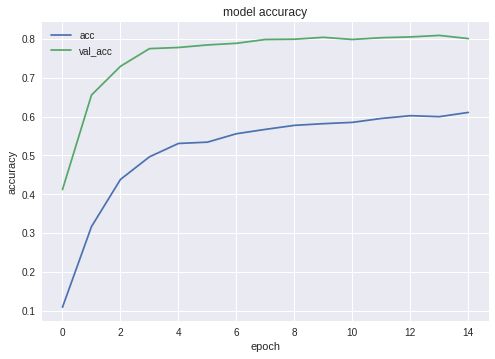
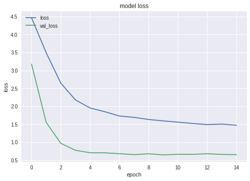
As you can see, the Network learns well.
After the training phase is complete, we need to perform testing; to do it, NN is presented with images it never saw. s you remember, we have put aside one image for each of dog species.
First, we need to load the NN. The reason is, exporting is a separate block of code, so we are likely to run it separately, without re-training the NN. As you use my code, you don't really care, but if you did your own development, you'd try to avoid retraining the same network one time after another.
For the same reason — this is somehow separate block of code — we are using additional includes here. Nothing prevents us from moving them up, of course:
A little testing, just to make sure we have loaded everything right:
Next thing, we need to get names of input and output layers of our network (unless we used «name» parameter when creating the network, which we did not).
We are going to use names of the input and output layer later, when importing the NN in Android Java application.
We can also use the following code to get this info:
However, first approach is preferred.
The following function exports Keras Neural Network to pb format, one that we are going to use in Android.
The last line prints the structure of our NN.
Exporting NN to Android app. is well formalized and should not pose any difficulties. There is, as usual, more than one way of doing it; we are going to use the most popular (at least, at the moment).
First of all, use Android Studio to create a new project. We are going to cut corners a little, so it will only contain a single activity.
As you can see, we have added «assets» folder and copied our Neural Network file there.
There are couple of changes we need to do to gradle file. First of all, we have to import the tensorflow-android library. It is used to handle Tensorflow (and Keras, accordingly) from Java:
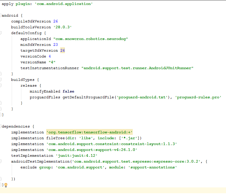
As an additional «hard to find» detail, note versions: versionCode and versionName. As you work on your app, you will need to upload new versions to Google Play. Without updating versions (something like 1 -> 2 -> 3...) you will not be able to do it.
First of all, our app. is going to be «heavy» — a 100 Mb Neural Network easily fits in memory of modern phones, but opening a separate instance of it every time the user «shares» an image from the Facebook is definitely not a good idea.
So we are going to make sure there is only one instance of our app:
By adding android:launchMode=«singleTask» to MainActivity, we tell Android to open an existing app, rather than launching another instance.
Then we make sure our app. shows up in a list of applications capable of handling shared images:
Finally, we need to request features and permissions, so the app can access system functionality it requires:
If you are familiar with Android programming, this part should raise no questions.
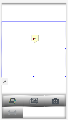
We are going to create two layouts, one for Portrait and one for Landscape mode. Here is the Portrait layout.
What we have here: a large view to show an image, a rather annoying list of commercials (shown when the «bone» button is pressed), «Help» buttons, buttons to load an image from File/Gallery and from Camera, and finally, an (initially hidden) button «Process».
In the activity itself we are going to implement some logic showing/hiding and enabling/disabling buttons depending on the state of the application.
The activity extends a standard Android Activity:
Let's take a look at code responcible for NN operations.
First of all, NN accepts a Bitmap. Originally it is a large Bitmap from file or Camera (m_bitmap), then we transform it to a standard 256x256 Bitmap (m_bitmapForNn). We also keep the image dimensions (256) in a constant:
We need to tell the NN what are the names for the input and output layers; if you consult the listing above, you'll find that names are (in our case! your case can be different!):
Then we declare the variable to hold TensofFlow object. Also, we store path to NN file in the assets:
Breeds of dogs, to present the user with a meaningful info, instead of indexes in the array:
Initially, we load a Bitmap. However, NN itself expects an array of RGB values, and its output is an array of probabilities ot the presented image being a particular breed. So we need to add two more arrays (note that 120 is number of breeds in our training dataset):
Load the tensorflow inference library
As NN's operation is a long one, we need to perform it in a separate thread, otherwise there is a good chance of hitting the system «app. not responding» warning, not to mention ruining the user experience.
In onCreate() of the MainActivity, we need to add the onClickListener for the «Process» button:
What the processImage() does is simply calling the thread we saw above:
We are not going to discuss UI-related code in this tutorial, as it is trivial and definitely is not part of «porting NN» task. However, there are few thing that should be clarified.
When we prevemted our app. from launching multiple instances, we have prevented, in the same time, a normal flow on control: if you share an image from Facebook, and then share another one, the application will not be restarted. It means that the «traditional» way of handling shared data by catching it in onCreate is not sufficient in our case, as onCreate is not called in a scenario we just created.
Here is a way to handle the situation:
1. In onCreate of MainActivity, call the onSharedIntent function:
Also, add a handler for onNewIntent:
The onSharedIntent function itself:
Now we either handle the shared image from onCreate (if the app was just started) or from onNewIntent if an instance was found in memory.
Good luck! If you like this article, please «like» it in social networks, also there are social buttons on a site itself.
However, there are still countless little details that… they are not insolvable, no. They simply take too much of your time, especially if you are a beginner. What would be of help is a step-by-step project, done right in front of you, start to end. A project that does not contain «this part is obvious so let's skip it» statements. Well, almost :)
In this tutorial we are going to walk through a Dog Breed Identifier: we will create and teach a Neural Network, then we will port it to Java for Android and publish on Google Play.
For those of you who want to see a end result, here is the link to NeuroDog App on Google Play.
Web site with my robotics: robotics.snowcron.com.
Web site with: NeuroDog User Guide.
Here is a screenshot of the program:
An overview
We are going to use Keras: Google's library for working with Neural Networks. It is high-level, which means that the learning curve will be steep, definitely faster than with other libraries I am aware of. Make yourself familiar with it: there are many high quality tutorials online.
We will use CNNs — Convolutional Neural Networks. CNNs (and more advanced networks based on them) are de-facto standard in image recognition. However, teaching one properly may become a formidable task: structure of the network, learning parameters (all those learning rates, momentums, L1 and L2 and so on) should be carefully adjusted, and as the task takes a lot of computational resources, we can not simply try all possible combinations.
This is one of the few reasons why in most cases we prefer using «transfer knowlege» to so-called «vanilla» approach. Transfer Knowlege uses a neural network trained by someone else (think Google) for some other task. Then we remove the last few layers of it, add layers of our own… and it works miracles.
It might sound strange: we took Google's network trained to recognize cats, flowers and furniture, and now it identifies breed of dogs! To understand how it works, let's take a look at the way Deep Neural Networks, including ones used for image recognition, work.
We feed it an image as the input. The first layer of a network analyses the image for simple patterns, like «short horizontal line», «an arch» and so on. The next layer takes these patterns (and where they are located on the image) and produces patterns of higher level, like «fur», «corner of an eye» etc. At the end, we have a puzzle that can be combined into a description of a dog: fur, two eyes, human leg in the mouth and so on.
Now, this all was done by a set of pre-trained layers we got (from Google or some other big player). Finally, we add our own layers on top of it and we teach it to work with those patterns to recognize breeds of dogs. Sounds logical.
To summarize, in this tutorial we are going to create «vanilla» CNN and couple of «transfer learning» networks of different types. As for «vanilla»: I am only going to use it as an example of how it can be done, but I am not going to fine-tune it, as «pre-trained» networks are way easier to use. Keras comes with few pre-trained networks, I'll choose couple of configurations and compare them.
As we want our Neural Network to be able to recognize dog breeds, we need to «show» it sample images of different breeds. Fortunately, there is a large dataset created for similar task (original here). In this article, I am going to use the version from Kaggle
Then I am going to port the «winner» to Android. Porting Keras NN to Android is relatively easy, and we are going to walk through all the required steps.
Then we will publish it on Google Play. As one should expect, Google is not going to cooperate, so few additional tricks will be required. For example, our Neural Network exceeds allowed size of Android APK: we will have to use bundle. Also, Google is not going to show our app in search results, unless we do certain magical things.
At the end we will have a fully working «commercial» (in quotes, as it is free though market-ready) Android NN-empowered application.
Development Environment
There are few different approaches to Keras programming, depending on the OS you use (Ubuntu is recommended), video card you have (or not) and so on. There is nothing wrong with configuring development environment on your local computer and installing all the necessary libraries and so on. Except… there is an easier way.
First, installing and configuring multiple development tools takes time and you will have to spend time again, when new versions become available. Second, training Neural Networks requires a lot of computational power. You can accelerate your computer by using GPU… at the moment of this writing, a top GPU for NN related computations costs 2000 — 7000 dollars. And configuring it takes time, too.
So we are going to use a different approach. See, Google allows people to use its GPUs free of charge for NN-related computations, it have also created a fully configured environment; all together it is called Google Colab. The service grants you access to a Jupiter Notebook with Python, Keras and tons of additional libraries already installed. All you need to do is to get a Google account (get a Gmail account, and you will have access to everything else) and that's it.
At the moment of this writing, Colab can be accessed by this link, but it can change. Just google up «Google Colab».
An obvious problem with Colab is that it is a WEB service. How are you going to access YOUR files from it? Saving Neural Networks after training is complete, loading data specific to your task and so on?
There are few (at the moment of this writing — three) different approaches; we are going to use what I believe is the best: using Google Drive.
Google Drive is a cloud storage that works pretty much as a hard drive, and it can be mapped to Google Colab (see code below). Then you work with it as you would with a local hard drive. So, for example, if you want to access photos of dogs from the Neural Network you created in Colab, you have to upload those photos to your Google Drive, that's all.
Creating and training the NN
Below, I am going to walk through the Python code, one block of code from Jupiter Notebook after another. You can copy that code to your notebook and run it, as blocks can be executed independent of each other.
Initialization
First of all, let's mount the Google Drive. Just two lines of code. That code needs to be executed only once per Colab session (say, once per six hours of work). If you run it the second time, it will be skipped as the drive is already mounted.
from google.colab import drive
drive.mount('/content/drive/')
The first time you will be asked to confirm the mounting — nothing complicated here. It looks like this:
>>> Go to this URL in a browser: ...
>>> Enter your authorization code:
>>> ··········
>>> Mounted at /content/drive/
A pretty standard include section; most likely some of the includes are not required. Also, as I am going to test different NN configurations, you will have to comment / uncomment some of them for a particular type of NNs: for example, to use InceptionV3 type NN, uncomment InceptionV3, and comment, say, ResNet50. Or not: you can keep those includes uncommented, it will use more memory, but that's all.
import datetime as dt
import pandas as pd
import seaborn as sns
import matplotlib.pyplot as plt
from tqdm import tqdm
import cv2
import numpy as np
import os
import sys
import random
import warnings
from sklearn.model_selection import train_test_split

import keras

from keras import backend as K
from keras import regularizers
from keras.models import Sequential
from keras.models import Model
from keras.layers import Dense, Dropout, Activation
from keras.layers import Flatten, Conv2D
from keras.layers import MaxPooling2D
from keras.layers import BatchNormalization, Input
from keras.layers import Dropout, GlobalAveragePooling2D
from keras.callbacks import Callback, EarlyStopping
from keras.callbacks import ReduceLROnPlateau
from keras.callbacks import ModelCheckpoint
import shutil
from keras.applications.vgg16 import preprocess_input
from keras.preprocessing import image
from keras.preprocessing.image import ImageDataGenerator

from keras.models import load_model

from keras.applications.resnet50 import ResNet50
from keras.applications.resnet50 import preprocess_input
from keras.applications.resnet50 import decode_predictions

from keras.applications import inception_v3
from keras.applications.inception_v3 import InceptionV3
from keras.applications.inception_v3
import preprocess_input as inception_v3_preprocessor

from keras.applications.mobilenetv2 import MobileNetV2

from keras.applications.nasnet import NASNetMobile
On Google Drive, we are going to create a folder for our files. The second line displays its content:
working_path = "/content/drive/My Drive/DeepDogBreed/data/"
!ls "/content/drive/My Drive/DeepDogBreed/data"

>>> all_images  labels.csv	models	test  train  valid
As you can see, photos of dogs (ones copied from Stanford dataset (see above) to Google Drive, are initially stored in all_images folder. Later on we are going to copy them to train, valid and test folders. We are going to save trained models in models folder. As for labels.csv file, it is part of a dataset, it maps image files to dog breeds.
There are many tests you can run to figure out what is it you have, let's run just one:
# Is GPU Working?
import tensorflow as tf
tf.test.gpu_device_name()
>>> '/device:GPU:0'
Ok, GPU is connected. If not, find it in Jupiter Notebook settings and turn it on.
Now we need to declare some constants we are going to use, like size of an image the Neural Network should expect and so on. Note, that we use 256x256 image, as this is large enough on one side and fits in memory in the other. However, some types of Neural Networks we are about to use are expecting 224x224 image. To handle this, when necessary, comment old image size and uncomment a new one.
Same approach (comment one — uncomment the other) applies to names of models we save, simply because we do not want to overwrite the result of a previous test when we try a new configuration.
warnings.filterwarnings("ignore")
os.environ['TF_CPP_MIN_LOG_LEVEL'] = '2'
np.random.seed(7)

start = dt.datetime.now()

BATCH_SIZE = 16
EPOCHS = 15
TESTING_SPLIT=0.3	# 70/30 %

NUM_CLASSES = 120
IMAGE_SIZE = 256

#strModelFileName = "models/ResNet50.h5"

# strModelFileName = "models/InceptionV3.h5"
strModelFileName = "models/InceptionV3_Sgd.h5"

#IMAGE_SIZE = 224
#strModelFileName = "models/MobileNetV2.h5"

#IMAGE_SIZE = 224
#strModelFileName = "models/NASNetMobileSgd.h5"
Loading data
First, let's load labels.csv file and split its content to training and validation parts. Note that there is no testing part yet, as I am going to cheat a bit, in order to get more data for training.
labels = pd.read_csv(working_path + 'labels.csv')
print(labels.head())

train_ids, valid_ids = train_test_split(labels,
	test_size = TESTING_SPLIT)

print(len(train_ids), 'train ids', len(valid_ids),
	'validation ids')
print('Total', len(labels), 'testing images')

>>>                                 id             breed
>>> 0  000bec180eb18c7604dcecc8fe0dba07       boston_bull
>>> 1  001513dfcb2ffafc82cccf4d8bbaba97             dingo
>>> 2  001cdf01b096e06d78e9e5112d419397          pekinese
>>> 3  00214f311d5d2247d5dfe4fe24b2303d          bluetick
>>> 4  0021f9ceb3235effd7fcde7f7538ed62  golden_retriever
>>> 7155 train ids 3067 validation ids
>>> Total 10222 testing images
Next thing, we need to copy the actual image files to training/validation/testing folders, according to array of file names we pass. The following function copies files with names provided to a folder specified.
def copyFileSet(strDirFrom, strDirTo, arrFileNames):
	arrBreeds = np.asarray(arrFileNames['breed'])
	arrFileNames = np.asarray(arrFileNames['id'])

	if not os.path.exists(strDirTo):
		os.makedirs(strDirTo)

	for i in tqdm(range(len(arrFileNames))):
		strFileNameFrom = strDirFrom +
			arrFileNames[i] + ".jpg"
		strFileNameTo = strDirTo + arrBreeds[i]
			+ "/" + arrFileNames[i] + ".jpg"

		if not os.path.exists(strDirTo + arrBreeds[i] + "/"):
			os.makedirs(strDirTo + arrBreeds[i] + "/")

			# As a new breed dir is created, copy 1st file
			# to "test" under name of that breed
			if not os.path.exists(working_path + "test/"):
				os.makedirs(working_path + "test/")

			strFileNameTo = working_path + "test/" + arrBreeds[i] + ".jpg"
			shutil.copy(strFileNameFrom, strFileNameTo)

		shutil.copy(strFileNameFrom, strFileNameTo)
As you can see, we only copy one file for each breed of dogs to a test folder. As we copy files, we also create subfolders — one subfolder per each breed of dogs. Images for each particular breed are copied into its subfolder.
The reason is, Keras can work with a directory structure organized this way, loading image files as they are needed, saving memory. It would be a very bad idea to load all 15,000 images into memory at once.
Calling this function every time we run our code would be an overkill: images are already copied, why should we copy them again. So, comment it out afret the first use:
# Move the data in subfolders so we can
# use the Keras ImageDataGenerator.
# This way we can also later use Keras
# Data augmentation features.

# --- Uncomment once, to copy files ---
#copyFileSet(working_path + "all_images/",
#    working_path + "train/", train_ids)
#copyFileSet(working_path + "all_images/",
#    working_path + "valid/", valid_ids)
Additionally, we need list of dog breeds:
breeds = np.unique(labels['breed'])
map_characters = {} #{0:'none'}
for i in range(len(breeds)):
  map_characters[i] = breeds[i]
  print("<item>" + breeds[i] + "</item>")

>>> <item>affenpinscher</item>
>>> <item>afghan_hound</item>
>>> <item>african_hunting_dog</item>
>>> <item>airedale</item>
>>> <item>american_staffordshire_terrier</item>
>>> <item>appenzeller</item>
Processing Images
We are going to use feature of Keras called ImageDataGenerators. ImageDataGenerator can process an image, resizing it, rotating, and so on. It can also take a processing function that does custom image manipulations.
def preprocess(img):
	img = cv2.resize(img,
		(IMAGE_SIZE, IMAGE_SIZE),
		interpolation = cv2.INTER_AREA)
	# or use ImageDataGenerator( rescale=1./255...

	img_1 = image.img_to_array(img)
	img_1 = cv2.resize(img_1, (IMAGE_SIZE, IMAGE_SIZE),
		interpolation = cv2.INTER_AREA)
	img_1 = np.expand_dims(img_1, axis=0) / 255.

	#img = cv2.blur(img,(5,5))

	return img_1[0]
Note the following line:
# or use ImageDataGenerator( rescale=1./255...
We can perform normalization (fitting image channel's 0-255 range to 0-1) in ImageDataGenerator itself. So why would we need preprocessor? As an example, I have provided the (commented out) blur function: that is a custom image manipulation. You can use anything from sharpening to HDR here.
We are going to use two different ImageDataGenerators, one for training and one for validation. The difference is, we need rotations and zooming for training, to make images more «diverse», but we do not need it for validation (not in this task).
train_datagen = ImageDataGenerator(
	preprocessing_function=preprocess,
	#rescale=1./255, # done in preprocess()
	# randomly rotate images (degrees, 0 to 30)
	rotation_range=30,
	# randomly shift images horizontally
	# (fraction of total width)
	width_shift_range=0.3,
	height_shift_range=0.3,
	# randomly flip images
	horizontal_flip=True,
	,vertical_flip=False,
	zoom_range=0.3)

val_datagen = ImageDataGenerator(
	preprocessing_function=preprocess)

train_gen = train_datagen.flow_from_directory(
	working_path + "train/",
	batch_size=BATCH_SIZE,
	target_size=(IMAGE_SIZE, IMAGE_SIZE),
	shuffle=True,
	class_mode="categorical")

val_gen = val_datagen.flow_from_directory(
	working_path + "valid/",
	batch_size=BATCH_SIZE,
	target_size=(IMAGE_SIZE, IMAGE_SIZE),
	shuffle=True,
	class_mode="categorical")
Creating Neural Network
As was mentioned above, we are going to create few types of Neural Networks. Each time we use a different function, different include library and in some cases, different image sizes. So to switch from one type of Neural Network to the other, you need to comment/uncomment corresponding code.
First, let's create «vanilla» CNN. It performs poorly, as I haven't optimized it, but at least it provides a framework you could use to create a network of your own (generally, it is a bad idea, as there are pre-trained networks available).
def createModelVanilla():
  model = Sequential()

  # Note the (7, 7) here. This is one of technics
  # used to reduce memory use by the NN: we scan
  # the image in a larger steps.
  # Also note regularizers.l2: this technic is
  # used to prevent overfitting. The "0.001" here
  # is an empirical value and can be optimized.
  model.add(Conv2D(16, (7, 7), padding='same',
	use_bias=False,
	input_shape=(IMAGE_SIZE, IMAGE_SIZE, 3),
	kernel_regularizer=regularizers.l2(0.001)))

  # Note the use of a standard CNN building blocks:
  # Conv2D - BatchNormalization - Activation
  # MaxPooling2D - Dropout
  # The last two are used to avoid overfitting, also,
  # MaxPooling2D reduces memory use.
  model.add(BatchNormalization(axis=3, scale=False))
  model.add(Activation("relu"))
  model.add(MaxPooling2D(pool_size=(2, 2),
	strides=(2, 2), padding='same'))
  model.add(Dropout(0.5))

  model.add(Conv2D(16, (3, 3), padding='same',
	use_bias=False,
	kernel_regularizer=regularizers.l2(0.01)))
  model.add(BatchNormalization(axis=3, scale=False))
  model.add(Activation("relu"))
  model.add(MaxPooling2D(pool_size=(2, 2),
	strides=(1, 1), padding='same'))
  model.add(Dropout(0.5))

  model.add(Conv2D(32, (3, 3), padding='same',
	use_bias=False,
	kernel_regularizer=regularizers.l2(0.01)))
  model.add(BatchNormalization(axis=3, scale=False))
  model.add(Activation("relu"))
  model.add(Dropout(0.5))

  model.add(Conv2D(32, (3, 3), padding='same',
	use_bias=False,
	kernel_regularizer=regularizers.l2(0.01)))
  model.add(BatchNormalization(axis=3, scale=False))
  model.add(Activation("relu"))
  model.add(MaxPooling2D(pool_size=(2, 2),
	strides=(1, 1), padding='same'))
  model.add(Dropout(0.5))

  model.add(Conv2D(64, (3, 3), padding='same',
	use_bias=False,
	kernel_regularizer=regularizers.l2(0.01)))
  model.add(BatchNormalization(axis=3, scale=False))
  model.add(Activation("relu"))
  model.add(Dropout(0.5))

  model.add(Conv2D(64, (3, 3), padding='same',
	use_bias=False,
	kernel_regularizer=regularizers.l2(0.01)))
  model.add(BatchNormalization(axis=3, scale=False))
  model.add(Activation("relu"))
  model.add(MaxPooling2D(pool_size=(2, 2),
	strides=(1, 1), padding='same'))
  model.add(Dropout(0.5))

  model.add(Conv2D(128, (3, 3), padding='same',
	use_bias=False,
	kernel_regularizer=regularizers.l2(0.01)))
  model.add(BatchNormalization(axis=3, scale=False))
  model.add(Activation("relu"))
  model.add(Dropout(0.5))

  model.add(Conv2D(128, (3, 3), padding='same',
	use_bias=False,
	kernel_regularizer=regularizers.l2(0.01)))
  model.add(BatchNormalization(axis=3, scale=False))
  model.add(Activation("relu"))
  model.add(MaxPooling2D(pool_size=(2, 2),
	strides=(1, 1), padding='same'))
  model.add(Dropout(0.5))

  model.add(Conv2D(256, (3, 3), padding='same',
	use_bias=False,
	kernel_regularizer=regularizers.l2(0.01)))
  model.add(BatchNormalization(axis=3, scale=False))
  model.add(Activation("relu"))
  model.add(Dropout(0.5))

  model.add(Conv2D(256, (3, 3), padding='same',
	use_bias=False,
	kernel_regularizer=regularizers.l2(0.01)))
  model.add(BatchNormalization(axis=3, scale=False))
  model.add(Activation("relu"))
  model.add(MaxPooling2D(pool_size=(2, 2),
	strides=(1, 1), padding='same'))
  model.add(Dropout(0.5))

  # This is the end on "convolutional" part of CNN.
  # Now we need to transform multidementional
  # data into one-dim. array for a fully-connected
  # classifier:
  model.add(Flatten())
  # And two layers of classifier itself (plus an
  # Activation layer in between):
  model.add(Dense(NUM_CLASSES, activation='softmax',
	kernel_regularizer=regularizers.l2(0.01)))
  model.add(Activation("relu"))
  model.add(Dense(NUM_CLASSES, activation='softmax',
	kernel_regularizer=regularizers.l2(0.01)))

  # We need to compile the resulting network.
  # Note that there are few parameters we can
  # try here: the best performing one is uncommented,
  # the rest is commented out for your reference.
  #model.compile(optimizer='rmsprop',
  #    loss='categorical_crossentropy',
  #    metrics=['accuracy'])
  #model.compile(
  #    optimizer=keras.optimizers.RMSprop(lr=0.0005),
  #    loss='categorical_crossentropy',
  #    metrics=['accuracy'])

  model.compile(optimizer='adam',
	loss='categorical_crossentropy',
	metrics=['accuracy'])
  #model.compile(optimizer='adadelta',
  #    loss='categorical_crossentropy',
  #    metrics=['accuracy'])

  #opt = keras.optimizers.Adadelta(lr=1.0,
  #    rho=0.95, epsilon=0.01, decay=0.01)
  #model.compile(optimizer=opt,
  #    loss='categorical_crossentropy',
  #    metrics=['accuracy'])

  #opt = keras.optimizers.RMSprop(lr=0.0005,
  #    rho=0.9, epsilon=None, decay=0.0001)
  #model.compile(optimizer=opt,
  #    loss='categorical_crossentropy',
  #    metrics=['accuracy'])

  # model.summary()

  return(model)
When we create Neural Network using transfer learning, the procedure changes:
def createModelMobileNetV2():
  # First, create the NN and load pre-trained
  # weights for it ('imagenet')
  # Note that we are not loading last layers of
  # the network (include_top=False), as we are
  # going to add layers of our own:
  base_model = MobileNetV2(weights='imagenet',
	include_top=False, pooling='avg',
	input_shape=(IMAGE_SIZE, IMAGE_SIZE, 3))

  # Then attach our layers at the end. These are
  # to build "classifier" that makes sense of
  # the patterns previous layers provide:
  x = base_model.output
  x = Dense(512)(x)
  x = Activation('relu')(x)
  x = Dropout(0.5)(x)

  predictions = Dense(NUM_CLASSES,
	activation='softmax')(x)

  # Create a model
  model = Model(inputs=base_model.input,
	outputs=predictions)

  # We need to make sure that pre-trained
  # layers are not changed when we train
  # our classifier:
  # Either this:
  #model.layers[0].trainable = False
  # or that:
  for layer in base_model.layers:
	layer.trainable = False

  # As always, there are different possible
  # settings, I tried few and chose the best:
  #  model.compile(optimizer='adam',
  #    loss='categorical_crossentropy',
  #    metrics=['accuracy'])
  model.compile(optimizer='sgd',
	loss='categorical_crossentropy',
	metrics=['accuracy'])

  #model.summary()

  return(model)
Creating other types of pre-trained NNs is very similar:
def createModelResNet50():
  base_model = ResNet50(weights='imagenet',
	include_top=False, pooling='avg',
	input_shape=(IMAGE_SIZE, IMAGE_SIZE, 3))

  x = base_model.output
  x = Dense(512)(x)
  x = Activation('relu')(x)
  x = Dropout(0.5)(x)

  predictions = Dense(NUM_CLASSES,
	activation='softmax')(x)

  model = Model(inputs=base_model.input,
	outputs=predictions)

  #model.layers[0].trainable = False

#  model.compile(loss='categorical_crossentropy',
#	optimizer='adam', metrics=['accuracy'])
  model.compile(optimizer='sgd',
	loss='categorical_crossentropy',
	metrics=['accuracy'])

  #model.summary()

  return(model)
Attn: the winner! This NN demonstrated the best results:
def createModelInceptionV3():
#  model.layers[0].trainable = False
#  model.compile(optimizer='sgd',
#    loss='categorical_crossentropy',
#    metrics=['accuracy'])

  base_model = InceptionV3(weights = 'imagenet',
	include_top = False,
	input_shape=(IMAGE_SIZE, IMAGE_SIZE, 3))

  x = base_model.output
  x = GlobalAveragePooling2D()(x)

  x = Dense(512, activation='relu')(x)
  predictions = Dense(NUM_CLASSES,
	activation='softmax')(x)

  model = Model(inputs = base_model.input,
	outputs = predictions)

  for layer in base_model.layers:
	layer.trainable = False

#  model.compile(optimizer='adam',
#    loss='categorical_crossentropy',
#    metrics=['accuracy'])
  model.compile(optimizer='sgd',
	loss='categorical_crossentropy',
	metrics=['accuracy'])

  #model.summary()

  return(model)
One more:
def createModelNASNetMobile():
#  model.layers[0].trainable = False
#  model.compile(optimizer='sgd',
#    loss='categorical_crossentropy',
#    metrics=['accuracy'])

  base_model = NASNetMobile(weights = 'imagenet',
	include_top = False,
	input_shape=(IMAGE_SIZE, IMAGE_SIZE, 3))

  x = base_model.output
  x = GlobalAveragePooling2D()(x)

  x = Dense(512, activation='relu')(x)
  predictions = Dense(NUM_CLASSES,
	activation='softmax')(x)

  model = Model(inputs = base_model.input,
	outputs = predictions)

  for layer in base_model.layers:
	layer.trainable = False

#  model.compile(optimizer='adam',
#	 loss='categorical_crossentropy',
#    metrics=['accuracy'])
  model.compile(optimizer='sgd',
	loss='categorical_crossentropy',
	metrics=['accuracy'])

  #model.summary()

  return(model)
Different types of NNs are used in different situations. In addition to precision issues, size maters (mobile NN is 5 times smaller than Inception one) and speed (if we need real time analysis of a video stream, we might have to sacrifice the precision).
Training the Neural Network
First of all, we are experimenting, so we need to be able to delete NNs we have saved before, but do not need anymore. The following function deletes NN if the file exists:
# Make sure that previous "best network" is deleted.
def deleteSavedNet(best_weights_filepath):
	if(os.path.isfile(best_weights_filepath)):
		os.remove(best_weights_filepath)
		print("deleteSavedNet():File removed")
	else:
		print("deleteSavedNet():No file to remove")
The way we create and delete NNs is straightforward. First, we delete. Now, if you don't wand to call delete, just remember that Jupiter Notebook has «run selection» function — select only what you need, and run it.
Then we create the NN if its file does not exist or load it if the file exists: of course, we can not call «delete» and then expect the NN to exist, so to use previously saved network, do not call delete.
In other words, we can create a new NN or use an existing one, depending on what we are experimenting right now. A simple scenario: we have trained the NN, then left for holiday. Google logged us out, so we need to re-load the NN: comment out the «delete» part and uncomment the «load» part.
deleteSavedNet(working_path + strModelFileName)
	#if not os.path.exists(working_path + "models"):
	#	os.makedirs(working_path + "models")
	#
	#if not os.path.exists(working_path +
	#	strModelFileName):
	# model = createModelResNet50()
	model = createModelInceptionV3()
	# model = createModelMobileNetV2()
	# model = createModelNASNetMobile()
	#else:
	#	model = load_model(working_path + strModelFileName)
Checkpoints are very important when teaching the NNs. You can create an array of functions to be called at the end of each training epoch, for example, you can save the NN if if shows better results than the last one saved.
checkpoint = ModelCheckpoint(working_path +
	strModelFileName, monitor='val_acc',
	verbose=1, save_best_only=True,
	mode='auto', save_weights_only=False)

callbacks_list = [ checkpoint ]
Finally, we will teach our NN using the training set:
# Calculate sizes of training and validation sets
STEP_SIZE_TRAIN=train_gen.n//train_gen.batch_size
STEP_SIZE_VALID=val_gen.n//val_gen.batch_size

# Set to False if we are experimenting with
# some other part of code, use history that
# was calculated before (and is still in
# memory
bDoTraining = True

if bDoTraining == True:
	# model.fit_generator does the actual training
	# Note the use of generators and callbacks
	# that were defined earlier
	history = model.fit_generator(generator=train_gen,
		steps_per_epoch=STEP_SIZE_TRAIN,
		validation_data=val_gen,
		validation_steps=STEP_SIZE_VALID,
		epochs=EPOCHS,
		callbacks=callbacks_list)

	# --- After fitting, load the best model
	# This is important as otherwise we'll
	# have the LAST model loaded, not necessarily
	# the best one.
	model.load_weights(working_path + strModelFileName)

	# --- Presentation part

	# summarize history for accuracy
	plt.plot(history.history['acc'])
	plt.plot(history.history['val_acc'])
	plt.title('model accuracy')
	plt.ylabel('accuracy')
	plt.xlabel('epoch')
	plt.legend(['acc', 'val_acc'], loc='upper left')
	plt.show()

	# summarize history for loss
	plt.plot(history.history['loss'])
	plt.plot(history.history['val_loss'])
	plt.title('model loss')
	plt.ylabel('loss')
	plt.xlabel('epoch')
	plt.legend(['loss', 'val_loss'], loc='upper left')
	plt.show()

	# As grid optimization of NN would take too long,
	# I did just few tests with different parameters.
	# Below I keep results, commented out, in the same
	# code. As you can see, Inception shows the best
	# results:

	# Inception:
	# adam: val_acc 0.79393
	# sgd: val_acc 0.80892

	# Mobile:
	# adam: val_acc 0.65290
	# sgd: Epoch 00015: val_acc improved from 0.67584 to 0.68469
	# sgd-30 epochs: 0.68

	# NASNetMobile, adam: val_acc did not improve from 0.78335
	# NASNetMobile, sgd: 0.8
Here are accuracy and loss charts for the winner NN:
As you can see, the Network learns well.
Testing the Neural Network
After the training phase is complete, we need to perform testing; to do it, NN is presented with images it never saw. s you remember, we have put aside one image for each of dog species.
# --- Test

j = 0

# Final cycle performs testing on the entire
# testing set.
for file_name in os.listdir(
	working_path + "test/"):
	img = image.load_img(working_path + "test/"
				+ file_name);

	img_1 = image.img_to_array(img)
	img_1 = cv2.resize(img_1, (IMAGE_SIZE, IMAGE_SIZE),
		interpolation = cv2.INTER_AREA)
	img_1 = np.expand_dims(img_1, axis=0) / 255.

	y_pred = model.predict_on_batch(img_1)

	# get 5 best predictions
	y_pred_ids = y_pred[0].argsort()[-5:][::-1]

	print(file_name)
	for i in range(len(y_pred_ids)):
		print("\n\t" + map_characters[y_pred_ids[i]]
			+ " ("
			+ str(y_pred[0][y_pred_ids[i]]) + ")")

	print("--------------------\n")

	j = j + 1
Exporting NN to Java
First, we need to load the NN. The reason is, exporting is a separate block of code, so we are likely to run it separately, without re-training the NN. As you use my code, you don't really care, but if you did your own development, you'd try to avoid retraining the same network one time after another.
# Test: load and run
model = load_model(working_path + strModelFileName)
For the same reason — this is somehow separate block of code — we are using additional includes here. Nothing prevents us from moving them up, of course:
from keras.models import Model
from keras.models import load_model
from keras.layers import *
import os
import sys
import tensorflow as tf
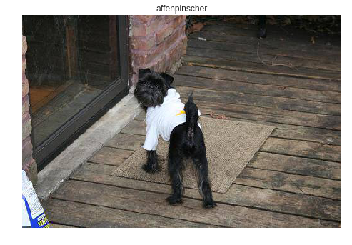
A little testing, just to make sure we have loaded everything right:
img = image.load_img(working_path
	+ "test/affenpinscher.jpg") #basset.jpg")
img_1 = image.img_to_array(img)
img_1 = cv2.resize(img_1,
	(IMAGE_SIZE, IMAGE_SIZE),
	interpolation = cv2.INTER_AREA)
img_1 = np.expand_dims(img_1, axis=0) / 255.

y_pred = model.predict(img_1)
Y_pred_classes = np.argmax(y_pred,axis = 1)
# print(y_pred)

fig, ax = plt.subplots()
ax.imshow(img)
ax.axis('off')
ax.set_title(map_characters[Y_pred_classes[0]])
plt.show()
Next thing, we need to get names of input and output layers of our network (unless we used «name» parameter when creating the network, which we did not).
model.summary()

>>> Layer (type)
>>> ======================
>>> input_7 (InputLayer)
>>> ______________________
>>> conv2d_283 (Conv2D)
>>> ______________________
>>> ...
>>> dense_14 (Dense)
>>> ======================
>>> Total params: 22,913,432
>>> Trainable params: 1,110,648
>>> Non-trainable params: 21,802,784
We are going to use names of the input and output layer later, when importing the NN in Android Java application.
We can also use the following code to get this info:
def print_graph_nodes(filename):
	g = tf.GraphDef()
	g.ParseFromString(open(filename, 'rb').read())
	print()
	print(filename)
	print("=======================INPUT===================")
	print([n for n in g.node if n.name.find('input') != -1])
	print("=======================OUTPUT==================")
	print([n for n in g.node if n.name.find('output') != -1])
	print("===================KERAS_LEARNING==============")
	print([n for n in g.node if n.name.find('keras_learning_phase') != -1])
	print("===============================================")
	print()

#def get_script_path():
#    return os.path.dirname(os.path.realpath(sys.argv[0]))
However, first approach is preferred.
The following function exports Keras Neural Network to pb format, one that we are going to use in Android.
def keras_to_tensorflow(keras_model, output_dir,
	model_name,out_prefix="output_",
		log_tensorboard=True):

	if os.path.exists(output_dir) == False:
		os.mkdir(output_dir)

	out_nodes = []

	for i in range(len(keras_model.outputs)):
		out_nodes.append(out_prefix + str(i + 1))
		tf.identity(keras_model.output[i],
			out_prefix + str(i + 1))

	sess = K.get_session()

	from tensorflow.python.framework import graph_util
	from tensorflow.python.framework graph_io

	init_graph = sess.graph.as_graph_def()

	main_graph =
		graph_util.convert_variables_to_constants(
			sess, init_graph, out_nodes)

	graph_io.write_graph(main_graph, output_dir,
		name=model_name, as_text=False)

	if log_tensorboard:
		from tensorflow.python.tools
			import import_pb_to_tensorboard

		import_pb_to_tensorboard.import_to_tensorboard(
			os.path.join(output_dir, model_name),
			output_dir)
Let's use these functions to create an exportes NN:
model = load_model(working_path
	+ strModelFileName)
keras_to_tensorflow(model,
	output_dir=working_path + strModelFileName,
	model_name=working_path + "models/dogs.pb")

print_graph_nodes(working_path + "models/dogs.pb")
The last line prints the structure of our NN.
Creating NN-empowered Android App
Exporting NN to Android app. is well formalized and should not pose any difficulties. There is, as usual, more than one way of doing it; we are going to use the most popular (at least, at the moment).
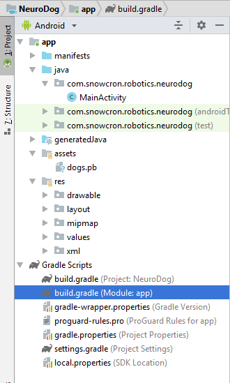
First of all, use Android Studio to create a new project. We are going to cut corners a little, so it will only contain a single activity.
As you can see, we have added «assets» folder and copied our Neural Network file there.
Gradle file
There are couple of changes we need to do to gradle file. First of all, we have to import the tensorflow-android library. It is used to handle Tensorflow (and Keras, accordingly) from Java:
As an additional «hard to find» detail, note versions: versionCode and versionName. As you work on your app, you will need to upload new versions to Google Play. Without updating versions (something like 1 -> 2 -> 3...) you will not be able to do it.
Manifest
First of all, our app. is going to be «heavy» — a 100 Mb Neural Network easily fits in memory of modern phones, but opening a separate instance of it every time the user «shares» an image from the Facebook is definitely not a good idea.
So we are going to make sure there is only one instance of our app:
<activity android:name=".MainActivity"
	android:launchMode="singleTask">
By adding android:launchMode=«singleTask» to MainActivity, we tell Android to open an existing app, rather than launching another instance.
Then we make sure our app. shows up in a list of applications capable of handling shared images:
<intent-filter>
	<!-- Send action required to display
		activity in share list -->
	<action android:name="android.intent.action.SEND" />

	<!-- Make activity default to launch -->
	<category android:name="android.intent.category.DEFAULT" />

	<!-- Mime type i.e. what can be shared with
		this activity only image and text -->
	<data android:mimeType="image/*" />
</intent-filter>
Finally, we need to request features and permissions, so the app can access system functionality it requires:
<uses-feature
	android:name="android.hardware.camera"
	android:required="true" />

<uses-permission android:name=
	"android.permission.WRITE_EXTERNAL_STORAGE" />
<uses-permission
	android:name="android.permission.READ_PHONE_STATE"
	tools:node="remove" />
If you are familiar with Android programming, this part should raise no questions.
Layout of the App.
We are going to create two layouts, one for Portrait and one for Landscape mode. Here is the Portrait layout.
What we have here: a large view to show an image, a rather annoying list of commercials (shown when the «bone» button is pressed), «Help» buttons, buttons to load an image from File/Gallery and from Camera, and finally, an (initially hidden) button «Process».
In the activity itself we are going to implement some logic showing/hiding and enabling/disabling buttons depending on the state of the application.
Main Activity
The activity extends a standard Android Activity:
public class MainActivity extends Activity
Let's take a look at code responcible for NN operations.
First of all, NN accepts a Bitmap. Originally it is a large Bitmap from file or Camera (m_bitmap), then we transform it to a standard 256x256 Bitmap (m_bitmapForNn). We also keep the image dimensions (256) in a constant:
static Bitmap m_bitmap = null;
static Bitmap m_bitmapForNn = null;

private int m_nImageSize = 256;
We need to tell the NN what are the names for the input and output layers; if you consult the listing above, you'll find that names are (in our case! your case can be different!):
private String INPUT_NAME = "input_7_1";
private String OUTPUT_NAME = "output_1";
Then we declare the variable to hold TensofFlow object. Also, we store path to NN file in the assets:
private TensorFlowInferenceInterface tf;
private String MODEL_PATH =
	"file:///android_asset/dogs.pb";
Breeds of dogs, to present the user with a meaningful info, instead of indexes in the array:
private String[] m_arrBreedsArray;
Initially, we load a Bitmap. However, NN itself expects an array of RGB values, and its output is an array of probabilities ot the presented image being a particular breed. So we need to add two more arrays (note that 120 is number of breeds in our training dataset):
private float[] m_arrPrediction = new float[120];
private float[] m_arrInput = null;
Load the tensorflow inference library
static
{
	System.loadLibrary("tensorflow_inference");
}
As NN's operation is a long one, we need to perform it in a separate thread, otherwise there is a good chance of hitting the system «app. not responding» warning, not to mention ruining the user experience.
class PredictionTask extends
	AsyncTask<Void, Void, Void>
{
	@Override
	protected void onPreExecute()
	{
		super.onPreExecute();
	}

	// ---

	@Override
	protected Void doInBackground(Void... params)
	{
		try
		{
			# We get RGB values packed in integers
			# from the Bitmap, then break those
			# integers into individual triplets

			m_arrInput = new float[
				m_nImageSize * m_nImageSize * 3];
			int[] intValues = new int[
				m_nImageSize * m_nImageSize];

			m_bitmapForNn.getPixels(intValues, 0,
				m_nImageSize, 0, 0, m_nImageSize,
				m_nImageSize);

			for (int i = 0; i < intValues.length; i++)
			{
				int val = intValues[i];
				m_arrInput[i * 3 + 0] =
					((val >> 16) & 0xFF) / 255f;
				m_arrInput[i * 3 + 1] =
					((val >> 8) & 0xFF) / 255f;
				m_arrInput[i * 3 + 2] =
					(val & 0xFF) / 255f;
			}

			// ---

			tf = new TensorFlowInferenceInterface(
				getAssets(), MODEL_PATH);

			//Pass input into the tensorflow
			tf.feed(INPUT_NAME, m_arrInput, 1,
				m_nImageSize, m_nImageSize, 3);

			//compute predictions
			tf.run(new String[]{OUTPUT_NAME}, false);

			//copy output into PREDICTIONS array
			tf.fetch(OUTPUT_NAME, m_arrPrediction);
		}
		catch (Exception e)
		{
			e.getMessage();
		}

		return null;
	}

	// ---

	@Override
	protected void onPostExecute(Void result)
	{
		super.onPostExecute(result);

		// ---

		enableControls(true);

		// ---

		tf = null;
		m_arrInput = null;

		# strResult contains 5 lines of text
		# with most probable dog breeds and
		# their probabilities
		m_strResult = "";

		# What we do below is sorting the array
		# by probabilities (using map)
		# and getting in reverse order) the
		# first five entries
		TreeMap<Float, Integer> map =
			new TreeMap<Float, Integer>(
				Collections.reverseOrder());
		for(int i = 0; i < m_arrPrediction.length;
			i++)
			map.put(m_arrPrediction[i], i);

		int i = 0;
		for (TreeMap.Entry<Float, Integer>
			pair : map.entrySet())
		{
			float key = pair.getKey();
			int idx = pair.getValue();

			String strBreed = m_arrBreedsArray[idx];

			m_strResult += strBreed + ": " +
				String.format("%.6f", key) + "\n";
			i++;
			if (i > 5)
				break;
		}

		m_txtViewBreed.setVisibility(View.VISIBLE);
		m_txtViewBreed.setText(m_strResult);
	}
}
In onCreate() of the MainActivity, we need to add the onClickListener for the «Process» button:
m_btn_process.setOnClickListener(new View.OnClickListener()
{
	@Override
	public void onClick(View v)
	{
		processImage();
	}
});
What the processImage() does is simply calling the thread we saw above:
private void processImage()
{
	try
	{
		enableControls(false);

		// ---

		PredictionTask prediction_task
			= new PredictionTask();
		prediction_task.execute();
	}
	catch (Exception e)
	{
		e.printStackTrace();
	}
}
Additional Details
We are not going to discuss UI-related code in this tutorial, as it is trivial and definitely is not part of «porting NN» task. However, there are few thing that should be clarified.
When we prevemted our app. from launching multiple instances, we have prevented, in the same time, a normal flow on control: if you share an image from Facebook, and then share another one, the application will not be restarted. It means that the «traditional» way of handling shared data by catching it in onCreate is not sufficient in our case, as onCreate is not called in a scenario we just created.
Here is a way to handle the situation:
1. In onCreate of MainActivity, call the onSharedIntent function:
protected void onCreate(
	Bundle savedInstanceState)
{
	super.onCreate(savedInstanceState);
	....
	onSharedIntent();
	....
Also, add a handler for onNewIntent:
@Override
protected void onNewIntent(Intent intent)
{
	super.onNewIntent(intent);
	setIntent(intent);

	onSharedIntent();
}
The onSharedIntent function itself:
private void onSharedIntent()
{
	Intent receivedIntent = getIntent();
	String receivedAction =
		receivedIntent.getAction();
	String receivedType = receivedIntent.getType();

	if (receivedAction.equals(Intent.ACTION_SEND))
	{
		// If mime type is equal to image
		if (receivedType.startsWith("image/"))
		{
			m_txtViewBreed.setText("");
			m_strResult = "";

			Uri receivedUri =
				receivedIntent.getParcelableExtra(
					Intent.EXTRA_STREAM);

			if (receivedUri != null)
			{
				try
				{
					Bitmap bitmap =
						MediaStore.Images.Media.getBitmap(
							this.getContentResolver(),
							receivedUri);

					if(bitmap != null)
					{
						m_bitmap = bitmap;
						m_picView.setImageBitmap(m_bitmap);
						storeBitmap();
						enableControls(true);
					}
				}
				catch (Exception e)
				{
					e.printStackTrace();
				}
			}
		}
	}
}
Now we either handle the shared image from onCreate (if the app was just started) or from onNewIntent if an instance was found in memory.
Good luck! If you like this article, please «like» it in social networks, also there are social buttons on a site itself.
