
Complex systems often appear chaotic or incomprehensible, yet closer examination reveals that such complexity can frequently be reduced to a simple underlying mechanism. By systematically removing layers of emergent behavior, one can uncover a fundamental rule or equation from which the entire system originates.
The work presented here is a translation and adaptation of my articles (Part 1, Part 2, Part 3, Part 4)
GitHub repository: billiard-fractals
The Billiard Fractals
While the system described in this article may appear trivial at first glance, the resulting patterns exhibit quasi-fractal behavior that can be analyzed, encoded, and even predicted through symbolic methods. The work presented here was developed independently through direct observation, rather than derived from prior literature.
A useful way to motivate this exploration is by analogy with a common physical phenomenon — wave interference. Consider waves on the surface of a river: a wavefront moves toward the shore, reflects, and overlaps with itself. Do these reflections contain an underlying order? Is it possible to extract structure from the interference?
To investigate this, we simplify the system. Rather than modeling the full wave, we consider only the motion vector — essentially, a ray. We also smooth the “shoreline” and discretize the environment into a rectangular grid. From this setup emerges the core construction of this article.
The example of waves on the surface of a river serves as a real, intuitive starting point — an accessible physical system that demonstrates how simple rules, such as reflection and interference, can produce complex behavior. It illustrates the central idea: that what appears chaotic often emerges from deterministic structure.
The initial motivation was driven by the conviction that apparent disorder is not randomness, but the result of unresolved or hidden structure. Any system that seems chaotic is governed by rules — its complexity a consequence of perspective, not unpredictability.
To explore this further, attention turned to constructing the simplest possible system that could look chaotic yet remain fully deterministic.
One such system involved a sine wave originating from the corner of a rectangle and reflecting off its boundaries. The nonlinearity of the sine function causes it to intersect itself in complex and unintuitive ways. However, due to limited tools available at the time, the model was simplified even further.
Instead of a sine wave, a straight line was used. The line was made periodic (dashed), and the system was designed to be reproducible using only a pencil and a sheet of graph paper. Despite its simplicity, this construction revealed intricate and structured patterns-forming the foundation of what would later be described as the “billiard fractals.”
Visualizing the Billiard Algorithm
The following sequence illustrates the core mechanism of the discrete billiard system:

An animated version:

Output pattern:

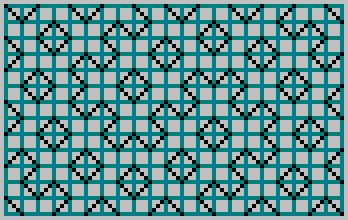
A selection of patterns generated from rectangles with various dimensions:
 |
 |
 |
 |
 |
 |
 |
 |
 |
 |
 |
 |
JavaScript implementation of this algorithm
pattern.js — source code
Fibonacci Numbers and Pattern Refinement
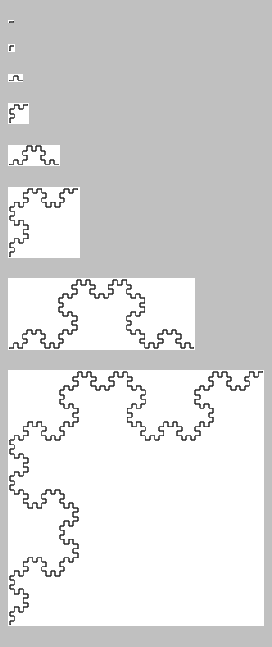
The patterns generated by this system exhibit fractal structure: they are self-similar across scales, recursive in construction, and can be compressed symbolically. As the rectangle dimensions increase following the Fibonacci sequence, the patterns reveal increasingly detailed versions of the same underlying structure.
This refinement process is simple: given rectangle dimensions (m, n), new dimensions are generated by Fibonacci summation. For example, starting with 8×13:
- 13 + 8 → 21 → becomes 13×21
- Then 21 + 13 → 34 → becomes 21×34, and so on
Each step increases resolution while preserving the underlying structure.
| 8×13 | 13×21 | 21×34 | 34×55 | 55×89 |
|---|---|---|---|---|
 |
 |
 |
 |
 |
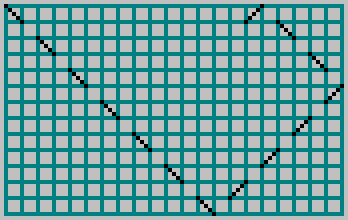
The article’s header image corresponds to the 233×377 pattern. Its structure can be directly compared with the earlier 13×21 case.
When constructing these patterns using Fibonacci-based dimensions, we are effectively approximating a rectangle with side lengths in the golden ratio — that is, a ratio approaching (1: φ). With each step, the approximation improves, and the pattern gains additional structure and resolution.
Although the overall structure of the pattern remains consistent during Fibonacci-based refinement, certain symmetries within the pattern depend on the parity of the rectangle's side lengths. Specifically, when both the width and height are odd integers, the resulting pattern exhibits clear diagonal, horizontal, and vertical symmetry. This occurs because the billiard path, under these conditions, terminates in the corner diagonally opposite from its starting point. In contrast, when one or both sides are even, the path terminates elsewhere, and the resulting pattern loses this precise symmetry — although the underlying recursive structure remains unchanged.
Boundary Analysis and Recursive Symmetry
To understand why the structure persists under Fibonacci expansion, consider cutting a square from the pattern. The boundary behavior reveals that the path (i.e., the “billiard ball”) always returns to its entry point:

Moreover, the path always (except for diagonal cases) crosses an even number of cells. This ensures that the pattern remains consistent across such subdivisions.

By recursively separating square regions from the larger pattern, the symbolic seed of the system can be exposed:

Binary Representation and Symbolic Extraction
The path traced by the billiard ball through the grid can be encoded as a binary sequence. As the ball moves from cell to cell, its internal state alternates according to a fixed rule. We can label these alternating states with binary values — for example, assigning 0 to one state and 1 to the other. This produces a binary field that can be visualized directly.
For example:


The top row of the binary field can be viewed as a symbolic boundary — a compact representation of the billiard system's behavior along a single edge. By studying the structure of the full 2D pattern and recursively extracting square sections from it, we arrive at symbolic generation rules. These rules allow us to reconstruct the boundary sequences using only binary operations.
Two core recursive generators are presented below:
function invers(array) {
    var temp = [];
    for (let i = 0; i < array.length; i++)
        temp[i] = array[i] === 0 ? 1 : 0;
    return temp;
}

function revers(array, s) {
    var temp = [];
    for (let i = 0; i < s; i++)
        temp[i] = array[array.length - i - 1];
    return temp;
}

function seqence(fn, fn1) {
    if (fn1 === 3) return [1];
    fn1 = fn - fn1;
    fn = fn - fn1;
    var array = seqence(fn, fn1);
    var a0 = invers(array);
    var a1 = (fn1 % 2 === 0) ? [1] : [];
    var a2 = revers(array, Math.floor((fn - fn1) / 2));
    return a0.concat(a1, a2);
}

function seqenceFibonacci(iterations) {
    let f0a = [0];
    let f1a = [0];
    for (let i = 0; i < iterations; i++) {
        let f0 = f0a.length;
        let a2 = revers(f1a, f0);
        if (f1a.length % 2 === 0) a2[0] ^= 1;
        f0a = f1a;
        f1a = f1a.concat(a2);
    }
    let array = [];
    for (let i = 0; i < Math.floor(f1a.length / 2); i++)
        array[i] = f1a[i * 2];
    return array;
}
These constructions reproduce the symbolic edges of Fibonacci-based patterns and can be interpreted as recursive encoding schemes derived directly from the observed geometry.
While the above generators are constructed specifically for Fibonacci-sized rectangles, preliminary experiments suggest that similar structures may emerge for other co-prime pairs. These systems may obey different symbolic transformation rules, but exhibit comparable recursive or compressible traits. A formal generalization of these behaviors remains an open area of exploration.
One of the central challenges that motivated the progression from the original 2013 construction to the deeper analysis in 2019 was the question of irrational proportions: what happens when the rectangle’s side lengths form a truly irrational ratio, such as (1: φ), rather than an integer-based approximation like 13: 21?
While recursive generators such as seqence(fn, fn1) accurately reproduced the symbolic boundary sequences for Fibonacci-based rectangles, they were inherently tied to integer dimensions. The challenge was clear: how can one generate the same structures when no exact grid alignment is possible — when the trajectory no longer closes?
This question defines the next stage of the investigation. To answer it, we will analyze the boundary sequences themselves — the so-called fractal sequences — and show how they encode the entire 2D pattern. We will show that these sequences — far from being edge artifacts — contain enough information to deterministically reconstruct the entire 2D pattern. This finding enables a powerful dimensional reduction: the entire billiard system can be expressed as a 1D sequence.
Binary Billiards
We now shift from the dashed-line visualization to a binary representation. Instead of drawing the trajectory, we color the cells the ball passes through, alternating black (0) and white (1) with each step.
Given a rectangle with side lengths  and
and  , the ball is launched from a corner and follows diagonal motion, reflecting off the walls. Each step alternates the internal binary state.
The reflection rule causes the pattern to shift by one cell after each bounce. This alternation creates a consistent visual structure.


When  and
and  are coprime, the trajectory visits every cell exactly once:

JavaScript implementation
binarypattern.js

If the dimensions share a common divisor ( ), the trajectory terminates at a corner before filling all cells:
In this case, the system is equivalent to a billiard in a reduced rectangle with dimensions ( ,
,  ):
):

Boundary Behavior and Symmetry
In the coprime case, the ball crosses every row and column. Notably, each pass between the top and left walls consists of an even number of steps.

From this, we can observe a critical symmetry: the left column contains the inverted bits of the top row, excluding the initial bit.

Furthermore, every second bit ( ) in the top sequence is the inverted version of its neighbor (
 ). Therefore, we can discard every second bit and retain full pattern information:
Halved sequence

For example, with dimensions  , the resulting sequence is: 1010010110
This sequence is unique for every coprime pair  . It encodes all necessary information about the pattern.
Sequence Interpretation
The trajectory between two reflections from the upper wall is always  cells long. Each such pass begins with a black cell (bit = 0) and ends with a white cell (bit = 1):

More formally:
- A bit of
1indicates that the ball arrived from a reflection off the right wall - A bit of
0indicates it came from the left wall
This mapping gives the sequence its meaning. In the diagram below, the trajectory is colored black when moving right and white when moving left:

A curious side effect of the billiard construction is that it naturally encodes binary division of two numbers. Specifically, by tracking the direction of the billiard ball’s movement at each wall collision, and sampling this information at exponentially increasing intervals, one can extract the binary digits of a rational fraction.
Let the billiard table have side lengths  and
and  , and let the ball bounce between corners. At each collision with the top or bottom wall:
If the ball is moving to the right, record a 0
If moving to the left, record a 1
Then, at every  -th collision (i.e., 1st, 2nd, 4th, 8th, …), we record the state.
Example: for a table of size  , we obtain:
1st  (bottom, →): 0
2nd  (top, ←):    1
4th  (top, →):    0
8th  (top, →):    0
16th (top, ←):    1
32nd (top, ←):    1
...
This produces the binary expansion:
0.1001111001111001111… Which is precisely the binary representation of  .
.
Reconstruction from the Sequence
The full billiard pattern can be reconstructed from this single boundary sequence. Even extrapolation beyond the grid is possible.
Let us begin by placing the bits along the top edge of a square grid of width  . Bits are spaced every 2 cells — these are the points where the ball would hit the upper wall:
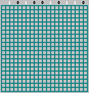
Then:
- If the bit is
1, we extend a diagonal to the left - If the bit is
0, we extend it to the right

The first bit (bit 0) is treated specially — it begins the pattern:
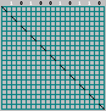
The reconstruction produces the exact original pattern:


JavaScript implementation
visualizer.js
This result shows that the 1D sequence contains complete information about the original 2D billiard pattern.
But we're not done.
From the surface of the river, we reduced the system to a rectangular billiard with a dashed diagonal trajectory. Then we reduced it further — to a binary field generated by alternating internal states. Now, we push the reduction one step further: we collapse the entire 2D billiard into a one-dimensional rule. A symbolic system with no geometry left — only structure.
This is where we begin to uncover the origin of these fractals.
One-dimensional billiards
On the  number axis, we take two points:
  and
and  .
.

Moving from one point to another, we measure the distances  :
:

We marked a point. We continue to measure the distance from this point, maintaining the direction. If we reach point  or
or  , we change the direction:

As you can see in the pictures above, the first point shows the place where the ball touches the bottom wall of the billiard table. We are not interested in this point. We will only mark the points  for
for  .
.
How to mark these points? Let's unfold our billiard table on the  axis. Let's mark the points
  . Now, having reached point
  , we do not change the direction of movement, but continue moving to point
  .
.
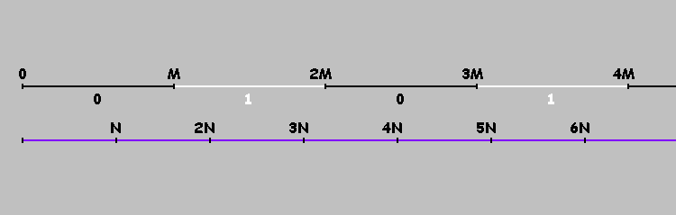
Points that are multiples of  divide our axis into segments. We will conditionally mark these segments with ones and zeros (alternating). On the segments marked with zeros, the ball (in rectangular billiards) moves from left to right. On the segments marked with ones, it moves from right to left. Or more simply: the ball moves from left to right if
  , for
, for

It is easy to see that the point at which the ball touched the upper wall of the billiard table is the remainder of dividing  by
by  . In this case, we don't need to record the movement of the ball in the opposite direction. We take the integer part of dividing
  by
by  , if it is even — we calculate the remainder of dividing
  by
by  . We divide the resulting remainder by 2 (the distance between adjacent touch points is two cells). This gives us the indices of the array elements that correspond to rightward motion (zeros). All other entries — representing leftward trajectories — are filled with ones.
Sequence length =  .
.
function sequence(m,n){
    var md=m/2;
    var array=[];
    for(var k=0;k<md;k++) array[k]=1;
    for(var k=0;k<md;k++) if(Math.floor(2*k*n/m)%2==0) array[((2*k*n)%m)/2]=0;
    return array;
}
Now we can build a binary sequence for billiards with any sides  and
and  (natural numbers). Some examples: 144x89 (Fibonacci numbers): 010100101101001011010110100101101001010010110101001011010100101
169x70 (Pell numbers): 010101101010010101101010010101101010100101011010101001010110101001010101010010101101010010
233x55 (odd Fibonacci numbers  and
and  ): 010010011011011001001101101100100100110110010010011011001001001101101100100110110110010010011011001001001101100100100
Very curious graphs are obtained if you take a billiard table with width  and construct sequences for each
  from
from  to
to  . Then these sequences are stacked.
    var array;
    for(var y=1;y<m;y++){
        array=sequence(m,y);
        for(var x=0;x<array.length;x++){
            if(array[x]==0) context.fillRect (x, y, 1, 1);
        }
    }
Some examples.
| M=610 | M=611 | M=612 | M=613 | M=614 |
|---|---|---|---|---|
 |
 |
 |
 |
 |
JavaScript implementation
sequences.js
We have sequences. How else can we visualize binary sequences? With Turtle graphics.
Turtle graphics
The sequence length determines the complexity of the curve. The more irrational the ratio between  and
and  , the more non-periodic and fractal — like the structure becomes.
Draw a segment. Then take bits from our sequence one by one. If bit = 1 — rotate the segment relative to the previous one by  (clockwise). If bit = 0 — rotate the segment by
  . The beginning of the next segment is the end of the previous one.

Take two large enough Fibonacci numbers:  and
and  . This ensures that the pattern is long enough for the fractal structure to become apparent, but still bounded enough for visualization.
We built the sequence: 0010110100101101001010010110100101101010010110100101101001010010110100101… (257114 symbols plus a zero bit).
Visualize using turtle graphics. The size of the initial segment is 1 pixels (the initial segment is in the lower right corner):

The next example is Pell numbers.
We take  and
and  .
.
The sequence is: 00101001010110101001010101010100101011010100101010110101001010101101 (235415 symbols plus a zero bit).
The size of the initial segment is 1 pixel:

Another example is the odd Fibonacci numbers  and
and  . Let's take
  and
and  . The sequence is: 00110110010010011011001001101101100100110110110010011011011001001… (158905 plus a zero bit). Instead of the angles
  and
and  , we will use the angles
  and
and  . The size of the initial segment is 1 pixels:

This curve is called "Fibonacci Word Fractal". The Hausdorff dimension for this curve is known:

JavaScript implementation
turtle.js
The problem unsolved yet.
Is it possible to draw a pattern for billiards, the sides of which are incommensurable (one of the sides is an irrational number)? At first glance, the task seems impossible. Trying to solve this problem, we will face a number of questions:
- If the sides are incommensurable, we cannot tile the billiards with cells of the same size.
- If the sides are incommensurable, the ball will infinitely reflect and will never get into the corner.
- Sequences in billiards are not filled in order, but chaotically.
The first two questions obviously have no solution. But if there were a way to fill the sequence in order, then we could, moving along the sequence from left to right, restore the pattern in the way we used above. And thus see what the pattern looks like in the upper left corner of the billiard table whose sides are incommensurable.
o_O
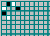
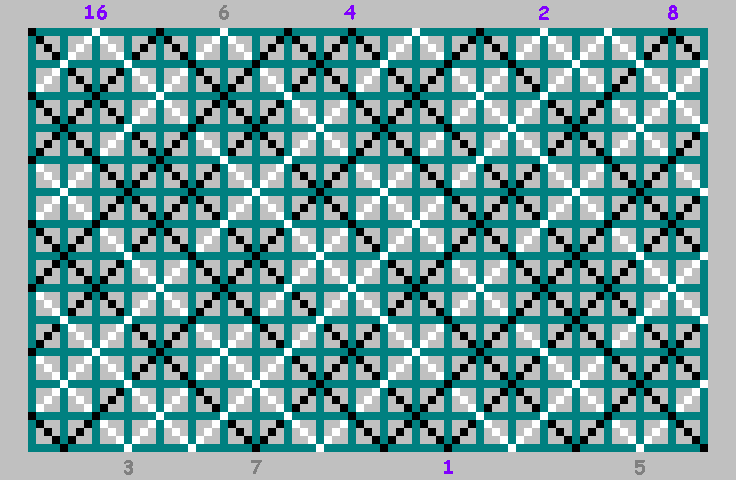
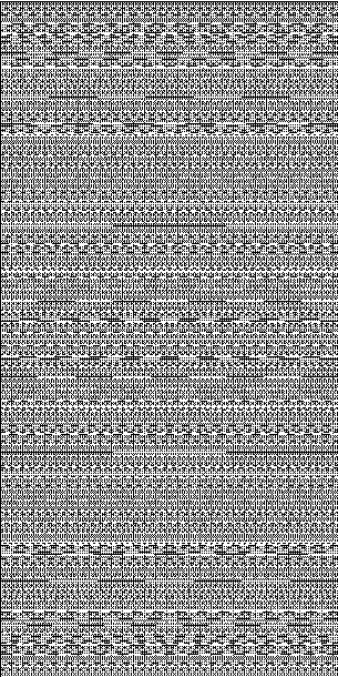
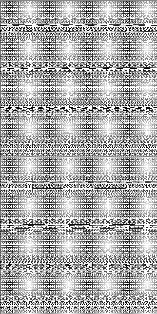
Let's take a billiard table, the sides of which are equal to the Fibonacci numbers (this trick may not work with other numbers). Let's throw a ball into it and record the number of times the ball touches the upper wall. We'll paint the numbers white if the ball moved from right to left and black if the ball moved from left to right:

White corresponds to the number one in the sequence, black to zero. Now let's arrange the numbers in order:
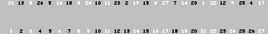
We've got exactly the same sequence of ones and zeros.
21(1), 13(0), 8(1), 26(0), 5(0), 16(1), 18(0), 3(1), 24(1), 10(0), 11(1), 23(0), 2(0), 19(1), 15(0), 6(1), 27(1), 7(0), 14(1), 20(0), 1(1), 22(1), 12(0), 9(1), 25(0), 4(0), 17(1)
1(1), 2(0), 3(1), 4(0), 5(0), 6(1), 7(0), 8(1), 9(1), 10(0), 11(1), 12(0), 13(0), 14(1), 15(0), 16(1), 17(1), 18(0), 19(1), 20(0), 21(1), 22(1), 23(0), 24(1), 25(0), 26(0), 27(1)
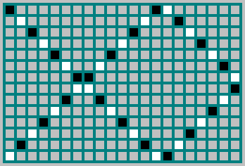
The origin is the upper left corner. The  axis is the width of the billiard table
  . The
. The  axis is the height of the billiard table
  . The numbers for which the sequences match are marked with white dots:

Numbers for which the sequence is inverted:
JavaScript implementation:
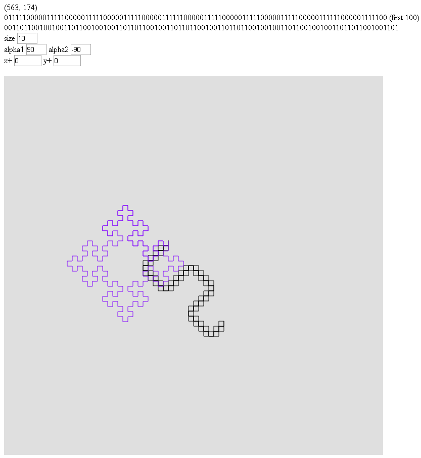
The first line is the mouse coordinates, which are used as the width and height of the billiard table.
The second line is the first 100 bits of the sequence obtained through the remainders of the division.
The third line is the first 100 bits of the sequence obtained through the parity of the integer part.
Black color — Visualization of the first sequence using Turtle graphics.
Purple — visualization of the second sequence.
JavaScript implementation
turtle_dynamic.js
In fact, in some cases, we do not need to take the remainder from the division. For Fibonacci numbers, it is enough to check the parity of the integer part of the division of  by
by  :
:

In the numerator we have  . In the denominator —
  .
.
As is known:

This gives us a bridge: rational billiards ( ,
,  ) converge toward an irrational limit —
  — allowing us to define an infinite symbolic sequence.
 is the Golden Ratio. An irrational number. Now we can write our formula as:

We have obtained a formula with which we can fill in the sequence for a billiard table, the width of which is  and the height is 1. The length of the sequence =
  , but we can restore part of the pattern by moving from left to right along the sequence and looking into the upper left corner of the billiard table. It remains to figure out how to calculate
One divided by the golden ratio can be rewritten as:

We can get rid of the two:

Our formula takes the form:

Now we can draw part of the billiard pattern with sides 1 and  :
:
If we do not subtract  each time, then every second bit in the sequence is inverted. We get the general formula:

Let's build a sequence for 
var x=2;
var q=[];
for(var k=0;k<256000;k++) q[k]=Math.floor(k*Math.sqrt(x))%2;
The first few bits of the sequence (A083035):
01001101100100110011001101100100110110011001001101100100110110…
Angles are  and
and  . The size of the initial segment is 5 pixels:

From this curve, we can reconstruct the "billiard pattern" and see what is around the curve:
It would be interesting to choose  and
and  for this pattern.
Number of segments in the repeating part of the curve =  (Pell numbers: 0, 1, 2, 5, 12, 29, 70, 169, 408, 985, 2378, … ).

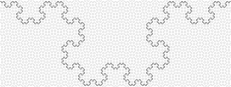
Someone may doubt that the parity of the integer part of  gives a fractal sequence. Let's visualize part of this sequence with the visualizer described earlier:

For clarity, I colored the longest curve in the resulting pattern:

This curve has a name — "Fibonacci word fractal".
Thus, by gradually reducing billiard geometry through symbolic encodings, we arrive at a powerful realization: even irrational systems, which defy spatial tiling and corner reflection, can still produce deterministic, fractal structure — using only integer math.
Filling the Fractal: From Symbolic Structure to Visual Density
In the previous sections, we showed how symbolic sequences can generate complex boundary structures in discrete 2D space. All of these patterns — whether generated by rational billiards or floor-based symbolic systems — form enclosed regions.
Some of these regions close against the boundaries of the rectangle, while others are fully self-contained, looping within the grid. In either case, the resulting trajectories always define fully enclosed cells.
Consider the following example:
A binary sequence generated by the floor function:

0100110110010011001001101100
Using the visualizer in diagonal mode, we generate a familiar fractal boundary.

However, switching to horizontal–vertical visualization, we invert every even-indexed bit and plot dashed lines accordingly. For bits with value 0, the lines are offset by one unit.
Vertical lines:

Horizontal lines:

Merged:

This technique resembles Hitomezashi stitching, a traditional Japanese method of generating textile patterns. While historically used to create decorative designs, this form of boundary generation bears striking similarity to the symbolic outlines produced in our system.
However, Hitomezashi does not solve the filling problem. It provides only the skeleton — the structure of edges — but no mechanism for interior construction.

A Symbolic Filling Algorithm
To solve this, we developed a symbolic method to automatically fill the interior regions — using only the original sequence. No region detection, no geometry, no search algorithms.
The method works as follows:
Construct a cumulative array a[n], based on the bitwise value of the fractal sequence:


In code:
var a = [0];
for (var i = 1; i < size; i++) {
    if (Math.floor(i * Math.sqrt(2)) % 2 == 1)
        a[i] = a[i - 1] + 1;
    else
        a[i] = a[i - 1] - 1;
}
Then, for each cell (x, y), compute:
q = (a[x] + a[y] + 512) % 4;
if (q === 0 || q === 1)
    context.fillRect(x, y, 1, 1);
The result is a filled pattern — not derived from pixel analysis or region marking, but emerging directly from the same symbolic system that generated the boundaries.
Full Algorithm
var a=[0];
for(var i=1;i<size;i++){
    if(Math.floor(i*Math.sqrt(2))%2==1)
        a[i]=a[i-1]+1;
    else
        a[i]=a[i-1]-1;
}
for(var x=0;x<size;x++){
    for(var y=0;y<size;y++){
        q=(a[x]+a[y]+512)%4;
        if(q==0 || q==1) context.fillRect(x, y, 1, 1);
    }
}
Examples
Fractal fill based on:


(Fibonacci-based)


Interactive
Visualizer — Fractal Fill from Irrationals
fractal.js
Dynamic Visualization — Using Rational Approximations
fractal_dynamic.js
We can compare fractal sequences from floor-based systems with sequences produced by a perfect shuffle function.
Here's our shuffle logic:
function shuffle(array, shiftAmount) {
    let len = array.length;
    let shuffled = new Array(len * 2);
    for (let i = 0; i < len; i++) {
        shuffled[2 * i] = array[(i + shiftAmount) % len];
        shuffled[2 * i + 1] = array[i];
    }
    return shuffled;
}
We start with a base array:
let array1 = [1, 0];
for (let i = 0; i < 15; i++) {
    array1 = shuffle(array1, (y + 45) * 128);
}
And compare it with this floor-based sequence:
let array2 = [];
for (let i = 0; i < sizexy; i++) {
    array2[i] = Math.floor(i * (y + 45) / 128) % 2;
}
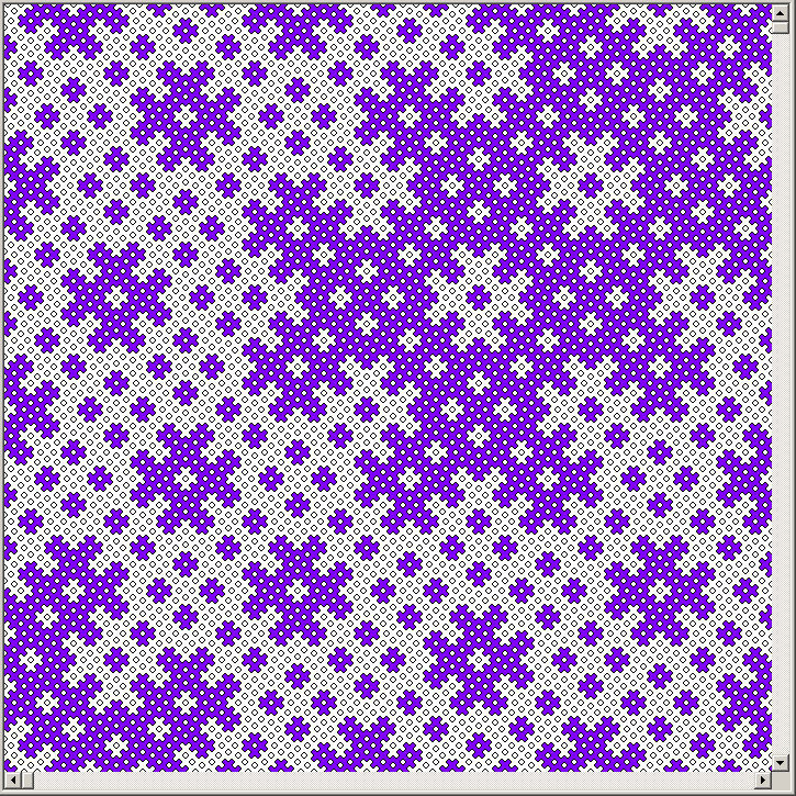
Both arrays are then visualized using our bit-pattern analysis:
for (let y = 0; y < sizexy; y++) {
    // generate array1 or array2

    let digit;
    let bits = [];
    for (let i = 0; i < len; i++) {
        digit = 0;
        for (let j = 0; j < bitLength; j++) {
            digit |= array[i + j] << (bitLength - 1 - j);
        }
        if (!bits.includes(digit)) {
            bits.push(digit);
        }
    }
    for (let i = 0; i < bits.length; i++) {
        context.fillRect(bits[i] * size, y * size, size, size);
    }
}
Here are the results:
Perfect shuffle:

Floor-based sequence:

The two patterns are visually identical.
This suggests that in some cases, perfect shuffle systems and irrational-floor systems may produce the same fractal binary sequences — or at least structurally equivalent ones.
We don’t yet have a formal proof or a unifying theory. But the match is too precise to ignore.
More analysis is needed to determine whether these overlaps are coincidence, mathematical identity, or reflections of a deeper shared structure. For now, we consider this a visually compelling anomaly — worth future investigation.
Nonlinear Functions and Symbolic Surface Slicing
Symbolic Rotation and the Circle Representation
The binary sequence generated by

can be interpreted geometrically as a rotation on the unit circle. At each step $k$, we rotate by an irrational angle (e.g., $\sqrt{2}$) and assign a 0 or 1 depending on which half of the circle the point lands in.
An alternative but mathematically equivalent formulation is:

The sine function is positive in one half of the circle and negative in the other — effectively producing the same binary threshold.

This circular diagram shows the orbit of
$$k \sqrt{2} \bmod 1$$
projected onto the unit circle. The points rotate continuously and never repeat. Each crossing of the horizontal axis (i.e., sign change of  ) causes a binary switch. The result is a Sturmian sequence — a symbolic encoding of irrational rotation — visualized as a point traveling clockwise and recording its hemisphere.
Interestingly, even a sequence like

generates a similarly complex structure. Though the function seems simple, stepping by exactly 1 radian per iteration is irrational with respect to the sine wave’s natural period of  . Thus:

Which means: irrational step size alone is enough to create symbolic fractals. It’s not the shape of the function — it’s the incommensurability that matters.
Geometric Interpretation of Linear Discretization
We begin with a geometric interpretation of the function

This can be visualized as a straight line  traversing a periodic 2D space where the
  -axis alternates between bands labeled 0 and 1. The value of the function at each step depends on the integer part of
  , determining whether the line intersects an even or odd band.

Alternatively, we may interpret the system as a function  with
with  acting as a discretization step along the vertical axis. This perspective reduces the behavior of the original billiard system to a symbolic sampling of a continuous linear function.
Both

serve as symbolic discretization methods — one yielding binary values via integer floor division, the other through sign thresholding on a continuous sinusoid.
Transition to Quadratic Functions
Having reduced the system to a linear function and its discretization, we now explore the effects of replacing the base function  with a nonlinear alternative.
Linear rotation yields symbolic Sturmian sequences. What happens if we increase the curvature? Quadratic growth is the simplest next step.
We now substitute the linear function with:

We construct the new sequence using:

q[x] = Math.floor(x * x * Math.sqrt(2)) % 2;
This substitution shifts us from uniform linear growth to a system governed by accelerating curvature, producing richer and more complex symbolic behavior.
Visualizing this sequence with the Symbolic Filling Algorithm yields a disordered pattern.


Similarly, applying Turtle graphics results in "chaotic" outputs

suggesting that the underlying symbolic dynamics differ significantly from the linear case. This observation motivated us to try a simpler visual encoding.
This prompts a reconsideration of visualization methods. Rather than relying on complex binary sequence encodings (e.g., symbolic filling or turtle graphics), we adopt a simpler approach:
- Place the first k elements of the sequence q[x] in the initial row.
- For each subsequent row along the y-axis, use q[x+ky].
- The result is a striking array of structured, interference-like patterns.
This reveals that a seemingly chaotic 1D sequence can exhibit coherent spatial behavior when unfolded along two dimensions. Generalizing this, we rewrite the indexing expression as:
q[x] = Math.floor((x + k * y) ** 2 * Math.sqrt(2)) % 2;
Expanding the square:

This quadratic form suggests a symbolic sampling of a 3D curved surface. We abstract this into a general expression:

Here:
 controls vertical scaling (the discretization frequency),
 introduces diagonal shear,
 modulates stretching along the
  -axis,
- and
 introduces curvature nonlinearity.
For example, setting  yields:

an elliptical paraboloid, a classic bowl-shaped surface.

We then visualize both:


...using this surface. Despite differing in output (binary vs. continuous), both render structurally equivalent patterns: the sine version produces smooth grayscale textures, while the floor function yields crisp binary segmentation. In either case, the resulting 2D images exhibit radial, interference-like motifs — strongly reminiscent of diffraction or holographic patterns.
| binary | continuous |
|---|---|
 |
 |
The sine-based rendering reveals finer gradients and smoother interference zones, but the underlying symbolic structure is identical to the binary version.
Holographic Analogy
In classical holography, a point source emits nested spherical wavefronts. When these are sliced by a flat recording plane, the amplitude at each (x, y) position encodes a continuous interference pattern. The spacing between wavefronts defines the wavelength — effectively a discretization step in the z-direction.
Our system inverts this paradigm: instead of slicing nested curved shells with a flat surface, we intersect a single curved surface with stacked, evenly spaced binary planes — symbolic layers representing a plane wavefront. Each (x, y) coordinate samples which symbolic layer the surface intersects, producing a binary (or thresholded) value.
While the components differ — continuous vs symbolic, curved emitter vs curved surface — the underlying mechanism is the same: a curved geometry intersected by layered structure, producing interference-like textures from simple spatial rules.
Despite differences in physical interpretation, both systems share a core structure: curved geometry meets layered slicing — and complexity emerges.
Our picture size is 400 pixels. We used  for previous picture to fit the picture.
Here another pattern with  :
:
| binary | continuous |
|---|---|
 |
 |
 modulates stretching along the
  -axis
-axis
(we will use continuous patterns from now).
 |
 |
|---|---|
 |
 |
 introduces diagonal shear
 |
 |
|---|---|
 |
 |
For  our equation becomes:

This is a hyperbolic paraboloid — a surface with negative Gaussian curvature:

 |
 |
|---|---|
 |
 |
For  our equation becomes:


 |
 |
 |
 |
 |
 |
 |
 |
The most interesting patterns are obtained if we take a  that differs slightly from 1. For example, for

 |
 |
 |
 |
 |
 |
 |
 |
 |
 |
 |
 |

 |
 |
 |
 |
Interactive
Dynamic Visualization — static
hologram_s.js
Dynamic Visualization — dynamic
hologram.js
Conclusion
This study began with a simple system: a billiard ball reflecting within a rectangular grid. By examining its trajectory and translating spatial behavior into symbolic sequences, we uncovered patterns exhibiting recursive structure, boundary self-similarity, and interference-like properties.
Through progressive abstraction — from 2D reflections to 1D symbolic sequences, and eventually to nonlinear surfaces — we showed that binary patterns can emerge from discretized irrational steps alone. Formulas such as:

generate deterministic sequences that yield quasi-fractal geometries when visualized spatially. Though entirely discrete, these systems exhibit behaviors commonly associated with continuous wave phenomena.
Further generalization using surface equations of the form:

reveals that curvature, shear, and nonlinearity shape the resulting symbolic slices in ways reminiscent of optical interference. The resemblance between these binary patterns and holographic textures suggests a structural parallel, despite their different origins.
No physical claims are made. However, the symbolic systems presented here demonstrate that simple integer-based operations, applied to irrational quantities or curved domains, can generate high-order structure with properties of both visual and mathematical interest. This offers a conceptual bridge between number theory, symbolic dynamics, and emergent spatial organization.
While this study has uncovered significant insights, several open questions remain to inspire further research:
- Generalization to Non-Fibonacci Ratios. The recursive generators presented here excel for Fibonacci-based rectangles, but can similar symbolic encoding schemes be developed for arbitrary co-prime pairs or other number sequences (e.g., Lucas numbers, Pell numbers)? What universal properties govern the resulting fractal structures?
- Irrational Billiards and Sequence Ordering. For billiard tables with incommensurable sides (e.g., 1: φ), we partially addressed pattern generation using floor-based sequences. However, can a robust method be devised to order these sequences consistently, enabling full reconstruction of the pattern in the absence of grid alignment?
- Perfect Shuffle and Floor-Based Equivalence. The striking similarity between perfect shuffle sequences and irrational floor-based sequences suggests a potential mathematical identity. Is there a formal equivalence between these systems, or do they converge only under specific conditions? What deeper structures might unify these approaches?
- Nonlinear Surface Generalizations. The transition to quadratic and higher-order surfaces produced rich, holographic-like patterns. How do variations in the exponent (d) or coefficients (a), (b), and © affect the fractal dimension or complexity of the resulting patterns? Can these be analytically quantified?
- Applications to Physical Systems. The visual resemblance to holographic interference patterns raises the question: can these symbolic systems model real-world wave phenomena, such as optical diffraction or quantum interference, in a computationally efficient way?
These questions highlight the potential for further exploration at the intersection of symbolic dynamics, fractal geometry, and computational visualization. By bridging discrete mathematics with continuous phenomena, this work offers a foundation for investigating how simple rules can encode complex, emergent behaviors — potentially extending to fields like number theory, physics, and computer graphics.
Symbolic sequences of the form:

exhibit fractal structure due to the interaction between irrational step sizes and discrete thresholds.
When extended to curved functions, such as:

the resulting binary fields begin to resemble interference patterns observed in wave-based systems.
Though entirely symbolic, these systems show a striking visual similarity to holographic interference textures. This suggests that certain nonlinear discretizations may encode symbolic analogs of wave behavior — hinting at a deeper structural correspondence between symbolic mathematics and wave-based physical systems.

